09 Exercises 2: WA state hourly data
Contents
09 Exercises 2: WA state hourly data#
UW Geospatial Data Analysis
CEE467/CEWA567
David Shean
import os
from glob import glob
import numpy as np
import xarray as xr
import pandas as pd
import geopandas as gpd
import cartopy.crs as ccrs
import matplotlib.pyplot as plt
#curr_y = pd.to_datetime("today").year
curr_y = 2022
Load the WA temperature, precipitation and snow depth products#
Note: these are extracted for 12:00 UTC
Really want daily averages for much of this, but I didn’t have time to go back and requery ERA5
Let’s use what we have to play around
era5_datadir = '/home/jovyan/jupyterbook/book/modules/09_NDarrays_xarray_ERA5/era5_data'
!ls -lh $era5_datadir
total 3.9G
-rw-r--r-- 1 jovyan users 2.0G Feb  4 05:48 1month_anomaly_Global_ea_2t.nc
-rw-r--r-- 1 jovyan users  48M Feb  4 05:48 climatology_0.25g_ea_2t.nc
-rw-r--r-- 1 jovyan users 1.9G Feb  4 05:48 WA_ERA5-Land_hourly_1950-2022_6hr.nc
merge_fn = os.path.join(era5_datadir, 'WA_ERA5-Land_hourly_1950-2022_6hr.nc')
Optional: start Dask cluster using Jupterlab interface, connect to client#
Please don’t use during lab session, but feel free to experiment on your own
Note this will use all CPUs on the shared node by default
#Start from Jupyterlab, copy paste corresponding code
#from dask.distributed import Client, LocalCluster
#cluster = LocalCluster()  # Launches a scheduler and workers locally
#client = Client(cluster)  # Connect to distributed cluster and override default
#Set up dask chunking
chunks = {'longitude':27, 'latitude':19}
wa_merge = xr.open_dataset(merge_fn, chunks=chunks)
wa_merge
<xarray.Dataset>
Dimensions:    (longitude: 81, latitude: 38, time: 105191)
Coordinates:
  * longitude  (longitude) float32 -124.8 -124.7 -124.6 ... -116.9 -116.8 -116.8
  * latitude   (latitude) float32 49.2 49.1 49.0 48.9 ... 45.8 45.7 45.6 45.5
  * time       (time) datetime64[ns] 1950-01-01T06:00:00 ... 2021-12-31T18:00:00
Data variables:
    t2m        (time, latitude, longitude) float32 dask.array<chunksize=(105191, 19, 27), meta=np.ndarray>
    sde        (time, latitude, longitude) float32 dask.array<chunksize=(105191, 19, 27), meta=np.ndarray>
    tp         (time, latitude, longitude) float32 dask.array<chunksize=(105191, 19, 27), meta=np.ndarray>
Attributes:
    Conventions:  CF-1.6
history: 2022-02-28 10:58:20 GMT by grib_to_netcdf-2.24.2: /opt/ecmw...wa_merge['t2m'] -= 273.15
wa_merge['t2m'].attrs['units'] = 'C'
#Convert meters to mm
wa_merge['tp'] *= 1000
wa_merge['tp'].attrs['units'] = 'mm'
wa_merge['t2m']
<xarray.DataArray 't2m' (time: 105191, latitude: 38, longitude: 81)>
dask.array<sub, shape=(105191, 38, 81), dtype=float32, chunksize=(105191, 19, 27), chunktype=numpy.ndarray>
Coordinates:
  * longitude  (longitude) float32 -124.8 -124.7 -124.6 ... -116.9 -116.8 -116.8
  * latitude   (latitude) float32 49.2 49.1 49.0 48.9 ... 45.8 45.7 45.6 45.5
  * time       (time) datetime64[ns] 1950-01-01T06:00:00 ... 2021-12-31T18:00:00
Attributes:
    units:      C
long_name: 2 metre temperaturewa_merge
<xarray.Dataset>
Dimensions:    (longitude: 81, latitude: 38, time: 105191)
Coordinates:
  * longitude  (longitude) float32 -124.8 -124.7 -124.6 ... -116.9 -116.8 -116.8
  * latitude   (latitude) float32 49.2 49.1 49.0 48.9 ... 45.8 45.7 45.6 45.5
  * time       (time) datetime64[ns] 1950-01-01T06:00:00 ... 2021-12-31T18:00:00
Data variables:
    t2m        (time, latitude, longitude) float32 dask.array<chunksize=(105191, 19, 27), meta=np.ndarray>
    sde        (time, latitude, longitude) float32 dask.array<chunksize=(105191, 19, 27), meta=np.ndarray>
    tp         (time, latitude, longitude) float32 dask.array<chunksize=(105191, 19, 27), meta=np.ndarray>
Attributes:
    Conventions:  CF-1.6
history: 2022-02-28 10:58:20 GMT by grib_to_netcdf-2.24.2: /opt/ecmw...#Unset units (avoid plotting in x and y label)
wa_merge['latitude'].attrs['units'] = None
wa_merge['longitude'].attrs['units'] = None
Clip to WA state geometry#
#wa_merge_clip = wa_merge.rio.write_crs(wa_state.crs);
#wa_merge_clip = wa_merge_clip.rio.clip(wa_geom, crs=world.crs, drop=False)
Compute seasonal mean values for each variable#
This may take ~30-60 seconds depending on chunks and server load
This is a simple
groupby()andmean()Inspect the output values - do these make sense?
wa_merge_seasonal_mean = wa_merge.groupby('time.season').mean().compute()
wa_merge_seasonal_mean
<xarray.Dataset>
Dimensions:    (longitude: 81, latitude: 38, season: 4)
Coordinates:
  * longitude  (longitude) float32 -124.8 -124.7 -124.6 ... -116.9 -116.8 -116.8
  * latitude   (latitude) float32 49.2 49.1 49.0 48.9 ... 45.8 45.7 45.6 45.5
  * season     (season) object 'DJF' 'JJA' 'MAM' 'SON'
Data variables:
    t2m        (season, latitude, longitude) float32 0.9609 0.2696 ... 6.214
    sde        (season, latitude, longitude) float32 0.2804 0.3006 ... 0.02896
    tp         (season, latitude, longitude) float32 5.971 5.626 ... 1.292 1.302
Attributes:
    Conventions:  CF-1.6
history: 2022-02-28 10:58:20 GMT by grib_to_netcdf-2.24.2: /opt/ecmw...#Hack to reorder seasons, as default is alphabetical
#order = np.array(['DJF', 'MAM', 'JJA', 'SON'], dtype=object)
order = np.array([0,2,1,3])
#wa_merge_seasonal_mean.season.values
wa_merge_seasonal_mean = wa_merge_seasonal_mean.isel(season=order)
#wa_merge_seasonal_resample = wa_merge.resample(time='Q-NOV').mean('time')
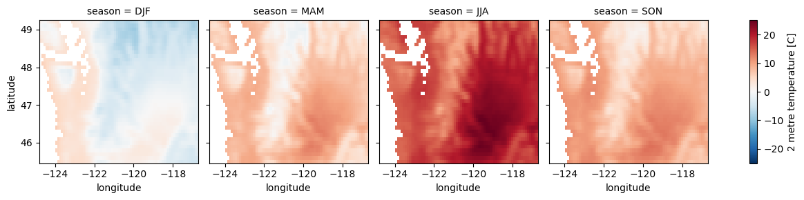
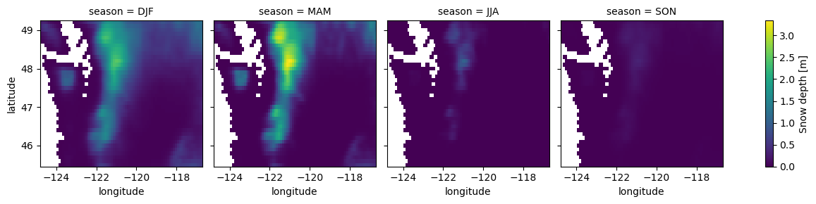
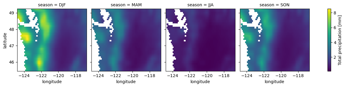
Plot seasonal mean grids#
Note that plot will assume
x='longitude', y='latitude', but can also explicitly specify
wa_merge_seasonal_mean.data_vars
Data variables:
    t2m      (season, latitude, longitude) float32 0.9609 0.2696 ... 6.408 6.214
    sde      (season, latitude, longitude) float32 0.2804 0.3006 ... 0.02896
    tp       (season, latitude, longitude) float32 5.971 5.626 ... 1.292 1.302
for i in wa_merge_seasonal_mean.data_vars:
    wa_merge_seasonal_mean[i].plot.imshow(col='season')
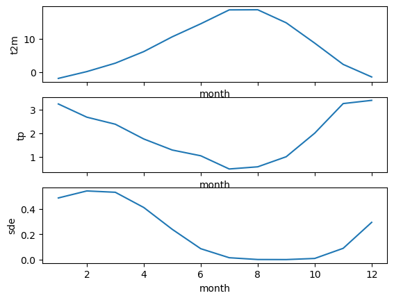
Compute mean monthly values for WA state#
wa_monthly_mean = wa_merge.groupby('time.month').mean('time').mean(['latitude','longitude']).compute()
wa_monthly_mean
<xarray.Dataset>
Dimensions:  (month: 12)
Coordinates:
  * month    (month) int64 1 2 3 4 5 6 7 8 9 10 11 12
Data variables:
    t2m      (month) float32 -1.957 0.09294 2.627 6.119 ... 8.671 2.257 -1.521
    sde      (month) float32 0.4876 0.5431 0.5326 ... 0.009246 0.08937 0.2947
tp (month) float32 3.241 2.678 2.378 1.75 ... 0.9946 1.997 3.257 3.394f, axa = plt.subplots(3,1, sharex=True)
wa_monthly_mean['t2m'].plot(ax=axa[0])
wa_monthly_mean['tp'].plot(ax=axa[1])
wa_monthly_mean['sde'].plot(ax=axa[2]);
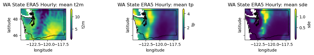
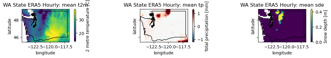
Helper function for plotting WA grids with state outline overlay#
def plotwa(ds_in, v_list=['t2m','tp','sde'], op='mean'):
    f,axa = plt.subplots(1,3, figsize=(12,2), sharex=True, sharey=True)
    for i,v in enumerate(v_list):
        ds_in[v].plot(ax=axa[i], robust=True)
        wa_state.plot(ax=axa[i], facecolor='none', edgecolor='black')
        axa[i].set_title('WA State ERA5 Hourly: %s %s' % (op, v))
    f.tight_layout()
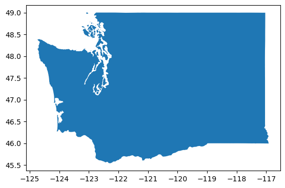
Get the WA state outline#
#states_url = 'http://eric.clst.org/assets/wiki/uploads/Stuff/gz_2010_us_040_00_5m.json'
states_url = 'http://eric.clst.org/assets/wiki/uploads/Stuff/gz_2010_us_040_00_500k.json'
states_gdf = gpd.read_file(states_url)
wa_state = states_gdf.loc[states_gdf['NAME'] == 'Washington']
wa_state.plot();
wa_geom = wa_state.iloc[0].geometry
wa_geom

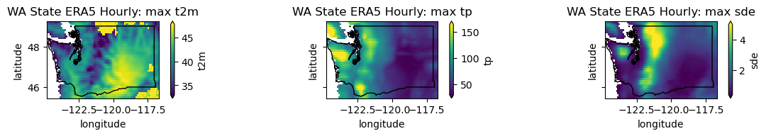
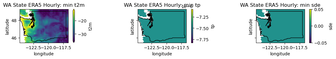
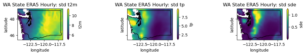
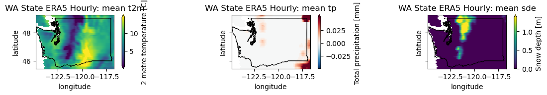
Create some plots of descriptive stats (mean, max, min, std) for 1979-present#
Pass the relevant dataset (e.g.
wa_merge.mean('time')) to theplotwahelper functionWhat do these metrics tell you?
What is causing most of the temperature variability captured by the std?
What is the highest temperature value
plotwa(wa_merge.mean('time'), op='mean')
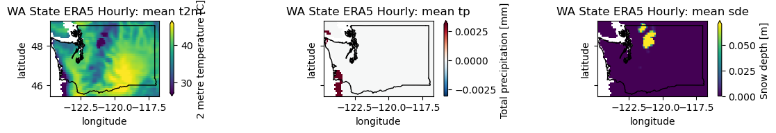
plotwa(wa_merge.max('time'), op='max')
plotwa(wa_merge.min('time'), op='min')
plotwa(wa_merge.std('time'), op='std')
/srv/conda/envs/notebook/lib/python3.10/site-packages/dask/array/numpy_compat.py:42: RuntimeWarning: invalid value encountered in divide
  x = np.divide(x1, x2, out)
Create a plot showing the conditions the day before and after the Mt. St. Helen’s eruption#
pre = wa_merge.sel(time='1980-05-17T06:00')
plotwa(pre)
post = wa_merge.sel(time='1980-05-19T06:00')
plotwa(post)
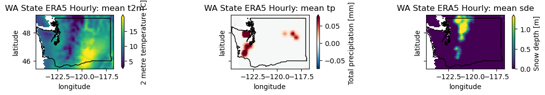
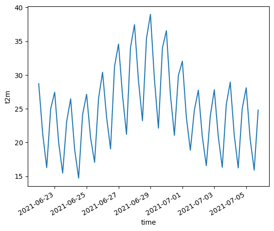
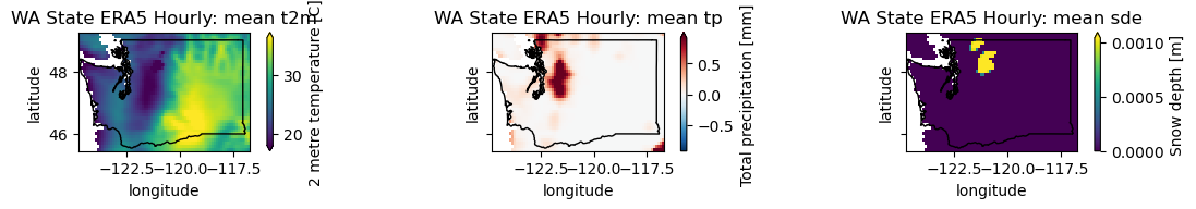
Create a plot showing the conditions during the June 2021 heat wave#
https://en.wikipedia.org/wiki/2021_Western_North_America_heat_wave
Extra credit: prepare a map of the long-term average t2m for June 29, then difference against the t2m values from June 29, 2021
wa_merge.t2m.sel(time=slice("2021-06-22", "2021-07-05")).mean(dim=('longitude', 'latitude')).plot()
[<matplotlib.lines.Line2D at 0x7f6ea48994e0>]
plotwa(wa_merge.sel(time='2021-06-24T00:00'))
plotwa(wa_merge.sel(time='2021-06-29T00:00'))
plotwa(wa_merge.sel(time='2021-07-03T00:00'))
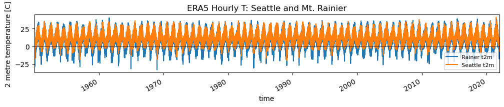
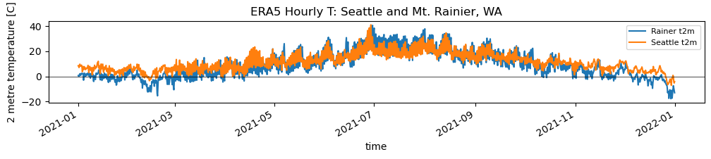
Extract the time series for Seattle and Mt. Rainier temperature and create line plot#
You’ll need to look up coordinates
Check the longitude system in the DataArrays (-180 to 180, or 0 to 360)
Can use the
sel()method to extract time series for the grid cell nearest the specified ‘longitude’ and ‘latitude’ coordinatesRemember, these are large grid cells (~31x31 km), so one grid cell could cover the most of Mt. Rainier (a single temperature value that includes the cold summit and the warmer, lowland river valleys)
Sanity check
#sea_coord = (-122.25, 47.5)
sea_coord = (-122.3321, 47.6062)
rainier_coord = (121.7603, 46.8523)
sea_ts = wa_merge.sel(longitude=sea_coord[0], latitude=sea_coord[1], method='nearest')
sea_ts
<xarray.Dataset>
Dimensions:    (time: 105191)
Coordinates:
    longitude  float32 -122.3
    latitude   float32 47.6
  * time       (time) datetime64[ns] 1950-01-01T06:00:00 ... 2021-12-31T18:00:00
Data variables:
    t2m        (time) float32 dask.array<chunksize=(105191,), meta=np.ndarray>
    sde        (time) float32 dask.array<chunksize=(105191,), meta=np.ndarray>
    tp         (time) float32 dask.array<chunksize=(105191,), meta=np.ndarray>
Attributes:
    Conventions:  CF-1.6
history: 2022-02-28 10:58:20 GMT by grib_to_netcdf-2.24.2: /opt/ecmw...rainier_ts = wa_merge.sel(longitude=rainier_coord[0], latitude=rainier_coord[1], method='nearest')
rainier_ts
<xarray.Dataset>
Dimensions:    (time: 105191)
Coordinates:
    longitude  float32 -116.8
    latitude   float32 46.9
  * time       (time) datetime64[ns] 1950-01-01T06:00:00 ... 2021-12-31T18:00:00
Data variables:
    t2m        (time) float32 dask.array<chunksize=(105191,), meta=np.ndarray>
    sde        (time) float32 dask.array<chunksize=(105191,), meta=np.ndarray>
    tp         (time) float32 dask.array<chunksize=(105191,), meta=np.ndarray>
Attributes:
    Conventions:  CF-1.6
history: 2022-02-28 10:58:20 GMT by grib_to_netcdf-2.24.2: /opt/ecmw...rainier_ts.time.values.min()
numpy.datetime64('1950-01-01T06:00:00.000000000')
f, ax = plt.subplots(figsize=(12,1.5))
v = 't2m'
rainier_ts[v].plot(ax=ax, label='Rainer %s' % v)
sea_ts[v].plot(ax=ax, label='Seattle %s' % v)
ax.axhline(0,color='k',lw=0.5)
ax.legend(fontsize=8)
ax.set_xlim(rainier_ts.time.values.min(), rainier_ts.time.values.max())
ax.set_title("ERA5 Hourly T: Seattle and Mt. Rainier");
f, ax = plt.subplots(figsize=(12,1.5))
v = 't2m'
rainier_ts[v].loc[f'{curr_y-1}-01-01':].plot(ax=ax, label='Rainer %s' % v)
sea_ts[v].loc[f'{curr_y-1}-01-01':].plot(ax=ax, label='Seattle %s' % v)
ax.axhline(0,color='k',lw=0.5)
ax.legend(fontsize=8)
ax.set_title("ERA5 Hourly T: Seattle and Mt. Rainier, WA");
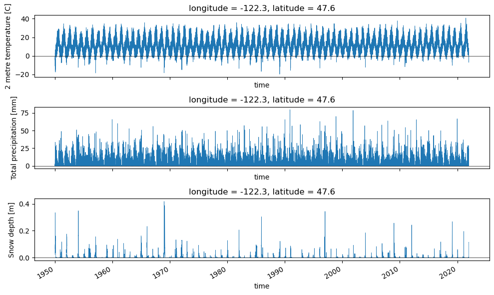
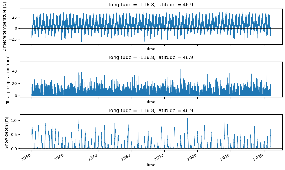
Helper function to plot time series#
def plotv(ds_in, v_list=['t2m','tp','sde']):
    f,axa = plt.subplots(3,1, figsize=(10,6), sharex=True)
    for i,v in enumerate(v_list):
        ds_in[v].dropna(dim='time').plot(ax=axa[i], lw=0.5)
        axa[i].axhline(0,color='k',lw=0.5)
    f.tight_layout()
plotv(wa_merge.sel(longitude=sea_coord[0], latitude=sea_coord[1], method='nearest'))
plotv(wa_merge.sel(longitude=rainier_coord[0], latitude=rainier_coord[1], method='nearest'))
Compute stats for monthly, annual time periods#
Can use
groupby('time.year').max(dim='time')Plot snow depth for April and September
Extra Credit: Create a map that shows the year containing the maximum T value at each grid cell#
These should mostly be in the most recent decade
Note the
.compute()is needed to converty dask array to ndarray for use in vectorized indexing
Note from 2022 - the ERA5-Land products include some cells that are all nan over time (e.g., ocean). This creates problems for the xarray argmax function, even with skipna=True, and various dropna calls
Need to revisit
#wa_merge['t2m'].dropna(dim='time', how='all').argmax(dim='time').compute()
#wa_merge['t2m'].idxmax(dim='time').compute()
#xr.apply_ufunc(np.nanargmax, wa_merge['t2m'].load())
#max_t_idx = wa_merge['t2m'].argmax(dim='time', skipna=True).compute()
#f, ax = plt.subplots()
#wa_merge['t2m']['time.year'][max_t_idx].plot(ax=ax)
#wa_state.plot(ax=ax, facecolor='none', edgecolor='black');
#wa_merge['t2m']['time.year'][max_t_idx].median()
Extra Credit#
Export one of the derived WA grids to rasterio#
Load SRTM DEM for WA#
Resample