08 Demo: SNOTEL Query and Download
Contents
08 Demo: SNOTEL Query and Download#
UW Geospatial Data Analysis
CEE467/CEWA567
David Shean
SNOTEL Introduction#
Read a bit about SNOTEL data for the Western U.S.:
https://www.nrcs.usda.gov/wps/portal/wcc/home/aboutUs/snowProgramOverview
https://www.nrcs.usda.gov/wps/portal/wcc/home/#elements=&networks=SNTL,SNTLT
This is actually a nice web interface, with some advanced querying and interactive visualization. You can also download formatted ASCII files (csv) for analysis. This is great for one-time projects, but it’s nice to have reproducible code that can be updated as new data appear, without manual steps. That’s what we’re going to do here.
About SNOTEL sites and data:#
https://www.nrcs.usda.gov/wps/portal/wcc/home/aboutUs/monitoringPrograms/automatedSnowMonitoring
https://directives.sc.egov.usda.gov/OpenNonWebContent.aspx?content=27630.wba
Check out the measurement information for Snow Depth sensor in Table 2-4
Sample plots for SNOTEL site at Paradise, WA (south side of Mt. Rainier)#
We will reproduce some of these plots/metrics during this lab
Interactive dashboard#
Snow today#


CUAHSI WOF server and automated Python data queries#
We are going to use a server set up by CUAHSI to serve the SNOTEL data, using a standardized database storage format and query structure. You don’t need to worry about this, but please quickly review the following:
Acronym soup#
SNOTEL = Snow Telemetry
CUAHSI = Consortium of Universities for the Advancement of Hydrologic Science, Inc
WOF = WaterOneFlow
WSDL = Web Services Description Language
USDA = United States Department of Agriculture
NRCS = National Resources Conservation Service
AWDB = Air-Water Database
Python options#
There are a few packages out there that offer convenience functions to query the online SNOTEL databases and unpack the results.
climata (https://pypi.org/project/climata/) - last commit Sept 2017 (not a good sign)
ulmo (https://github.com/ulmo-dev/ulmo) - last commit Sept 2021 (will be superseded by a package called Quest, but still maintained by Emilio Mayorga over at UW APL)
You can also write your own queries using the Python requests module and some built-in XML parsing libraries.
Hopefully not overwhelming amount of information - let’s just go with ulmo for now. I’ve done most of the work to prepare functions for querying and processing the data. Once you wrap your head around all of the acronyms, it’s pretty simple, basically running a few functions here: https://ulmo.readthedocs.io/en/latest/api.html#module-ulmo.cuahsi.wof
We will use ulmo with daily data for this exercise, but please feel free to experiment with hourly data, other variables or other approaches to fetch SNOTEL data.
ulmo installation#
Note that
ulmois not part of the default Hub environmentWe will cover more on conda and environment management in coming weeks, but know that you can temporarily install packages from terminal or even in Jupyterhub notebook
When running conda install from notebook, make sure to use the
-yflag to avoid interactive prompt
Note that packages installed this way won’t persist when your server is shut down, so you will need to reinstall to use again
Fortunately, once we’ve used ulmo for data access and download, we won’t need it again
#Doesn't work until ulmo is installed
#import ulmo
#Install directly from github repo main branch
#%pip install git+https://github.com/ulmo-dev/ulmo.git
#!python -m pip install git+https://github.com/ulmo-dev/ulmo.git
#!conda install -q -u ulmo
!mamba install -q -y ulmo
import ulmo
import os
import numpy as np
import matplotlib.pyplot as plt
import pandas as pd
import geopandas as gpd
from shapely.geometry import Point
#Create local directory to store images
datadir = 'snotel_data'
if not os.path.exists(datadir):
    os.makedirs(datadir)
Load state polygons for later use#
states_url = 'http://eric.clst.org/assets/wiki/uploads/Stuff/gz_2010_us_040_00_5m.json'
#states_url = 'http://eric.clst.org/assets/wiki/uploads/Stuff/gz_2010_us_040_00_500k.json'
states_gdf = gpd.read_file(states_url)
CUAHSI WOF server information#
Try typing this in a browser, note what you get back (xml)
#http://his.cuahsi.org/wofws.html
wsdlurl = 'https://hydroportal.cuahsi.org/Snotel/cuahsi_1_1.asmx?WSDL'
ulmo.cuahsi.wof.get_sites?
Signature:
ulmo.cuahsi.wof.get_sites(
    wsdl_url,
    suds_cache=('default',),
    timeout=None,
    user_cache=False,
)
Docstring:
Retrieves information on the sites that are available from a WaterOneFlow
service using a GetSites request.  For more detailed information including
which variables and time periods are available for a given site, use
``get_site_info()``.

Parameters
----------
wsdl_url : str
    URL of a service's web service definition language (WSDL) description.
    All WaterOneFlow services publish a WSDL description and this url is the
    entry point to the service.
suds_cache : `None` or tuple
    SOAP local cache duration for WSDL description and client object.
    Pass a cache duration tuple like ('days', 3) to set a custom duration.
    Duration may be in months, weeks, days, hours, or seconds.
    If unspecified, the default duration (1 day) will be used.
    Use ``None`` to turn off caching.
timeout : int or float
    suds SOAP URL open timeout (seconds).
    If unspecified, the suds default (90 seconds) will be used.
user_cache : bool
    If False (default), use the system temp location to store cache WSDL and
    other files. Use the default user ulmo directory if True.

Returns
-------
sites_dict : dict
    a python dict with site codes mapped to site information
File:      /srv/conda/envs/notebook/lib/python3.10/site-packages/ulmo/cuahsi/wof/core.py
Type:      function
Run the query for available sites#
sites = ulmo.cuahsi.wof.get_sites(wsdlurl)
If you get an error (AttributeError: module 'ulmo' has no attribute 'cuahsi'), you need to restart your kernel and “Run All Above Selected Cell”
Take a moment to inspect the output#
What is the
type?Note data structure and different key/value pairs for each site
type(sites)
dict
#Preview first item in dictionary
next(iter(sites.items()))
('SNOTEL:301_CA_SNTL',
 {'code': '301_CA_SNTL',
  'name': 'Adin Mtn',
  'network': 'SNOTEL',
  'location': {'latitude': '41.2358283996582',
   'longitude': '-120.79192352294922'},
  'elevation_m': '1886.7120361328125',
  'site_property': {'county': 'Modoc',
   'state': 'California',
   'site_comments': 'beginDate=10/1/1983 12:00:00 AM|endDate=1/1/2100 12:00:00 AM|HUC=180200021403|HUD=18020002|TimeZone=-8.0|actonId=20H13S|shefId=ADMC1|stationTriplet=301:CA:SNTL|isActive=True',
   'pos_accuracy_m': '0'}})
Store as a Pandas DataFrame called sites_df#
See the
from_dictfunctionUse
orientoption so the sites comprise the DataFrame index, with columns for ‘name’, ‘elevation_m’, etcUse the
dropnamethod to remove any empty records
sites_df = pd.DataFrame.from_dict(sites, orient='index').dropna()
sites_df.head()
| code | name | network | location | elevation_m | site_property | |
|---|---|---|---|---|---|---|
| SNOTEL:301_CA_SNTL | 301_CA_SNTL | Adin Mtn | SNOTEL | {'latitude': '41.2358283996582', 'longitude': ... | 1886.7120361328125 | {'county': 'Modoc', 'state': 'California', 'si... |
| SNOTEL:907_UT_SNTL | 907_UT_SNTL | Agua Canyon | SNOTEL | {'latitude': '37.522171020507813', 'longitude'... | 2712.719970703125 | {'county': 'Kane', 'state': 'Utah', 'site_comm... |
| SNOTEL:916_MT_SNTL | 916_MT_SNTL | Albro Lake | SNOTEL | {'latitude': '45.59722900390625', 'longitude':... | 2529.840087890625 | {'county': 'Madison', 'state': 'Montana', 'sit... |
| SNOTEL:1267_AK_SNTL | 1267_AK_SNTL | Alexander Lake | SNOTEL | {'latitude': '61.749668121337891', 'longitude'... | 48.768001556396484 | {'county': 'Matanuska-Susitna', 'state': 'Alas... |
| SNOTEL:908_WA_SNTL | 908_WA_SNTL | Alpine Meadows | SNOTEL | {'latitude': '47.779571533203125', 'longitude'... | 1066.800048828125 | {'county': 'King', 'state': 'Washington', 'sit... |
Clean up the DataFrame and prepare Point geometry objects#
We covered this with the GLAS data conversion to GeoPandas
Convert
'location'column (contains dictionary with'latitude'and'longitude'values) to ShapelyPointobjectsStore as a new
'geometry'columnDrop the
'location'column, as this is no longer neededUpdate the
dtypeof the'elevation_m'column to float
sites_df['location']
SNOTEL:301_CA_SNTL     {'latitude': '41.2358283996582', 'longitude': ...
SNOTEL:907_UT_SNTL     {'latitude': '37.522171020507813', 'longitude'...
SNOTEL:916_MT_SNTL     {'latitude': '45.59722900390625', 'longitude':...
SNOTEL:1267_AK_SNTL    {'latitude': '61.749668121337891', 'longitude'...
SNOTEL:908_WA_SNTL     {'latitude': '47.779571533203125', 'longitude'...
                                             ...
SNOTEL:877_AZ_SNTL     {'latitude': '33.812419891357422', 'longitude'...
SNOTEL:1228_UT_SNTL    {'latitude': '39.132331848144531', 'longitude'...
SNOTEL:1197_UT_SNTL    {'latitude': '37.747970581054688', 'longitude'...
SNOTEL:878_WY_SNTL     {'latitude': '43.9322509765625', 'longitude': ...
SNOTEL:1033_CO_SNTL    {'latitude': '40.794879913330078', 'longitude'...
Name: location, Length: 930, dtype: object
sites_df['geometry'] = [Point(float(l['longitude']), float(l['latitude'])) for l in sites_df['location']]
sites_df = sites_df.drop(columns='location')
sites_df = sites_df.astype({"elevation_m":float})
Review output#
Take a moment to familiarize yourself with the DataFrame structure and different columns.
Note that the index is a set of strings with format ‘SNOTEL:1000_OR_SNTL’
Extract the first record with
locReview the
'site_property'dictionary
sites_df.head()
| code | name | network | elevation_m | site_property | geometry | |
|---|---|---|---|---|---|---|
| SNOTEL:301_CA_SNTL | 301_CA_SNTL | Adin Mtn | SNOTEL | 1886.712036 | {'county': 'Modoc', 'state': 'California', 'si... | POINT (-120.79192352294922 41.2358283996582) |
| SNOTEL:907_UT_SNTL | 907_UT_SNTL | Agua Canyon | SNOTEL | 2712.719971 | {'county': 'Kane', 'state': 'Utah', 'site_comm... | POINT (-112.27117919921875 37.52217102050781) |
| SNOTEL:916_MT_SNTL | 916_MT_SNTL | Albro Lake | SNOTEL | 2529.840088 | {'county': 'Madison', 'state': 'Montana', 'sit... | POINT (-111.95902252197266 45.59722900390625) |
| SNOTEL:1267_AK_SNTL | 1267_AK_SNTL | Alexander Lake | SNOTEL | 48.768002 | {'county': 'Matanuska-Susitna', 'state': 'Alas... | POINT (-150.88966369628906 61.74966812133789) |
| SNOTEL:908_WA_SNTL | 908_WA_SNTL | Alpine Meadows | SNOTEL | 1066.800049 | {'county': 'King', 'state': 'Washington', 'sit... | POINT (-121.69847106933594 47.779571533203125) |
sites_df.loc['SNOTEL:301_CA_SNTL']
code                                                   301_CA_SNTL
name                                                      Adin Mtn
network                                                     SNOTEL
elevation_m                                            1886.712036
site_property    {'county': 'Modoc', 'state': 'California', 'si...
geometry              POINT (-120.79192352294922 41.2358283996582)
Name: SNOTEL:301_CA_SNTL, dtype: object
sites_df.loc['SNOTEL:301_CA_SNTL']['site_property']
{'county': 'Modoc',
 'state': 'California',
 'site_comments': 'beginDate=10/1/1983 12:00:00 AM|endDate=1/1/2100 12:00:00 AM|HUC=180200021403|HUD=18020002|TimeZone=-8.0|actonId=20H13S|shefId=ADMC1|stationTriplet=301:CA:SNTL|isActive=True',
 'pos_accuracy_m': '0'}
Explode the site_property and site_comments fields#
These are nested dictionary objects and strings with either | or = delimiters
site_property_df = pd.json_normalize(sites_df['site_property'])
site_property_df
| county | state | site_comments | pos_accuracy_m | |
|---|---|---|---|---|
| 0 | Modoc | California | beginDate=10/1/1983 12:00:00 AM|endDate=1/1/21... | 0 |
| 1 | Kane | Utah | beginDate=10/1/1994 12:00:00 AM|endDate=1/1/21... | 0 |
| 2 | Madison | Montana | beginDate=9/1/1996 12:00:00 AM|endDate=1/1/210... | 0 |
| 3 | Matanuska-Susitna | Alaska | beginDate=8/28/2014 12:00:00 AM|endDate=1/1/21... | 0 |
| 4 | King | Washington | beginDate=9/1/1994 12:00:00 AM|endDate=1/1/210... | 0 |
| ... | ... | ... | ... | ... |
| 925 | Gila | Arizona | beginDate=12/1/1938 12:00:00 AM|endDate=1/1/21... | 0 |
| 926 | Sanpete | Utah | beginDate=10/1/2012 12:00:00 AM|endDate=1/1/21... | 0 |
| 927 | Iron | Utah | beginDate=10/1/2012 12:00:00 AM|endDate=1/1/21... | 0 |
| 928 | Park | Wyoming | beginDate=10/1/1979 12:00:00 AM|endDate=1/1/21... | 0 |
| 929 | Jackson | Colorado | beginDate=8/14/2002 6:00:00 AM|endDate=1/1/210... | 0 |
930 rows × 4 columns
#Extract site_comments column names
site_comments_names = [x.split('=')[0] for x in site_property_df['site_comments'].iloc[0].split('|')]
#Split using both delimiters and preserve every other record
site_comments_df = site_property_df['site_comments'].str.split('\||=', expand=True).iloc[:,1::2]
site_comments_df = site_comments_df.set_axis(site_comments_names, axis=1, copy=False)
site_comments_df
| beginDate | endDate | HUC | HUD | TimeZone | actonId | shefId | stationTriplet | isActive | |
|---|---|---|---|---|---|---|---|---|---|
| 0 | 10/1/1983 12:00:00 AM | 1/1/2100 12:00:00 AM | 180200021403 | 18020002 | -8.0 | 20H13S | ADMC1 | 301:CA:SNTL | True |
| 1 | 10/1/1994 12:00:00 AM | 1/1/2100 12:00:00 AM | 160300020301 | 16030002 | -8.0 | 12M26S | AGUU1 | 907:UT:SNTL | True |
| 2 | 9/1/1996 12:00:00 AM | 1/1/2100 12:00:00 AM | 100200050701 | 10020005 | -8.0 | 11D28S | ABRM8 | 916:MT:SNTL | True |
| 3 | 8/28/2014 12:00:00 AM | 1/1/2100 12:00:00 AM | 190205051106 | -9.0 | 50M01S | ALXA2 | 1267:AK:SNTL | True | |
| 4 | 9/1/1994 12:00:00 AM | 1/1/2100 12:00:00 AM | 171100100501 | 17110010 | -8.0 | 21B48S | APSW1 | 908:WA:SNTL | True |
| ... | ... | ... | ... | ... | ... | ... | ... | ... | ... |
| 925 | 12/1/1938 12:00:00 AM | 1/1/2100 12:00:00 AM | 150601030802 | 15060103 | -8.0 | 10S01S | WKMA3 | 877:AZ:SNTL | True |
| 926 | 10/1/2012 12:00:00 AM | 1/1/2100 12:00:00 AM | 140600090303 | 14060009 | -8.0 | 11K32S | WRIU1 | 1228:UT:SNTL | True |
| 927 | 10/1/2012 12:00:00 AM | 1/1/2100 12:00:00 AM | 160300060202 | 16030006 | -8.0 | 12M11S | YKEU1 | 1197:UT:SNTL | True |
| 928 | 10/1/1979 12:00:00 AM | 1/1/2100 12:00:00 AM | 100800130103 | 10080013 | -8.0 | 09F18S | YOUW4 | 878:WY:SNTL | True |
| 929 | 8/14/2002 6:00:00 AM | 1/1/2100 12:00:00 AM | 101800010202 | 10180001 | -8.0 | 06J19S | ZIRC2 | 1033:CO:SNTL | True |
930 rows × 9 columns
#Combine the site_properites and the site_comments dataframes
site_property_df = pd.concat([site_property_df.drop('site_comments', axis=1), site_comments_df], axis=1)
site_property_df
| county | state | pos_accuracy_m | beginDate | endDate | HUC | HUD | TimeZone | actonId | shefId | stationTriplet | isActive | |
|---|---|---|---|---|---|---|---|---|---|---|---|---|
| 0 | Modoc | California | 0 | 10/1/1983 12:00:00 AM | 1/1/2100 12:00:00 AM | 180200021403 | 18020002 | -8.0 | 20H13S | ADMC1 | 301:CA:SNTL | True |
| 1 | Kane | Utah | 0 | 10/1/1994 12:00:00 AM | 1/1/2100 12:00:00 AM | 160300020301 | 16030002 | -8.0 | 12M26S | AGUU1 | 907:UT:SNTL | True |
| 2 | Madison | Montana | 0 | 9/1/1996 12:00:00 AM | 1/1/2100 12:00:00 AM | 100200050701 | 10020005 | -8.0 | 11D28S | ABRM8 | 916:MT:SNTL | True |
| 3 | Matanuska-Susitna | Alaska | 0 | 8/28/2014 12:00:00 AM | 1/1/2100 12:00:00 AM | 190205051106 | -9.0 | 50M01S | ALXA2 | 1267:AK:SNTL | True | |
| 4 | King | Washington | 0 | 9/1/1994 12:00:00 AM | 1/1/2100 12:00:00 AM | 171100100501 | 17110010 | -8.0 | 21B48S | APSW1 | 908:WA:SNTL | True |
| ... | ... | ... | ... | ... | ... | ... | ... | ... | ... | ... | ... | ... |
| 925 | Gila | Arizona | 0 | 12/1/1938 12:00:00 AM | 1/1/2100 12:00:00 AM | 150601030802 | 15060103 | -8.0 | 10S01S | WKMA3 | 877:AZ:SNTL | True |
| 926 | Sanpete | Utah | 0 | 10/1/2012 12:00:00 AM | 1/1/2100 12:00:00 AM | 140600090303 | 14060009 | -8.0 | 11K32S | WRIU1 | 1228:UT:SNTL | True |
| 927 | Iron | Utah | 0 | 10/1/2012 12:00:00 AM | 1/1/2100 12:00:00 AM | 160300060202 | 16030006 | -8.0 | 12M11S | YKEU1 | 1197:UT:SNTL | True |
| 928 | Park | Wyoming | 0 | 10/1/1979 12:00:00 AM | 1/1/2100 12:00:00 AM | 100800130103 | 10080013 | -8.0 | 09F18S | YOUW4 | 878:WY:SNTL | True |
| 929 | Jackson | Colorado | 0 | 8/14/2002 6:00:00 AM | 1/1/2100 12:00:00 AM | 101800010202 | 10180001 | -8.0 | 06J19S | ZIRC2 | 1033:CO:SNTL | True |
930 rows × 12 columns
#Combine with the original sites dataframe
sites_df_all = pd.concat([sites_df.drop('site_property', axis=1), site_property_df.set_index(sites_df.index)], axis=1)
#Extract Hydrologic Unit region and basin codes (HUC2 and HUC6)
sites_df_all['HUC2'] = sites_df_all['HUC'].str[0:2]
sites_df_all['HUC6'] = sites_df_all['HUC'].str[0:6]
sites_df_all
| code | name | network | elevation_m | geometry | county | state | pos_accuracy_m | beginDate | endDate | HUC | HUD | TimeZone | actonId | shefId | stationTriplet | isActive | HUC2 | HUC6 | |
|---|---|---|---|---|---|---|---|---|---|---|---|---|---|---|---|---|---|---|---|
| SNOTEL:301_CA_SNTL | 301_CA_SNTL | Adin Mtn | SNOTEL | 1886.712036 | POINT (-120.79192352294922 41.2358283996582) | Modoc | California | 0 | 10/1/1983 12:00:00 AM | 1/1/2100 12:00:00 AM | 180200021403 | 18020002 | -8.0 | 20H13S | ADMC1 | 301:CA:SNTL | True | 18 | 180200 |
| SNOTEL:907_UT_SNTL | 907_UT_SNTL | Agua Canyon | SNOTEL | 2712.719971 | POINT (-112.27117919921875 37.52217102050781) | Kane | Utah | 0 | 10/1/1994 12:00:00 AM | 1/1/2100 12:00:00 AM | 160300020301 | 16030002 | -8.0 | 12M26S | AGUU1 | 907:UT:SNTL | True | 16 | 160300 |
| SNOTEL:916_MT_SNTL | 916_MT_SNTL | Albro Lake | SNOTEL | 2529.840088 | POINT (-111.95902252197266 45.59722900390625) | Madison | Montana | 0 | 9/1/1996 12:00:00 AM | 1/1/2100 12:00:00 AM | 100200050701 | 10020005 | -8.0 | 11D28S | ABRM8 | 916:MT:SNTL | True | 10 | 100200 |
| SNOTEL:1267_AK_SNTL | 1267_AK_SNTL | Alexander Lake | SNOTEL | 48.768002 | POINT (-150.88966369628906 61.74966812133789) | Matanuska-Susitna | Alaska | 0 | 8/28/2014 12:00:00 AM | 1/1/2100 12:00:00 AM | 190205051106 | -9.0 | 50M01S | ALXA2 | 1267:AK:SNTL | True | 19 | 190205 | |
| SNOTEL:908_WA_SNTL | 908_WA_SNTL | Alpine Meadows | SNOTEL | 1066.800049 | POINT (-121.69847106933594 47.779571533203125) | King | Washington | 0 | 9/1/1994 12:00:00 AM | 1/1/2100 12:00:00 AM | 171100100501 | 17110010 | -8.0 | 21B48S | APSW1 | 908:WA:SNTL | True | 17 | 171100 |
| ... | ... | ... | ... | ... | ... | ... | ... | ... | ... | ... | ... | ... | ... | ... | ... | ... | ... | ... | ... |
| SNOTEL:877_AZ_SNTL | 877_AZ_SNTL | Workman Creek | SNOTEL | 2103.120117 | POINT (-110.91773223876953 33.81241989135742) | Gila | Arizona | 0 | 12/1/1938 12:00:00 AM | 1/1/2100 12:00:00 AM | 150601030802 | 15060103 | -8.0 | 10S01S | WKMA3 | 877:AZ:SNTL | True | 15 | 150601 |
| SNOTEL:1228_UT_SNTL | 1228_UT_SNTL | Wrigley Creek | SNOTEL | 2842.869629 | POINT (-111.35684967041016 39.13233184814453) | Sanpete | Utah | 0 | 10/1/2012 12:00:00 AM | 1/1/2100 12:00:00 AM | 140600090303 | 14060009 | -8.0 | 11K32S | WRIU1 | 1228:UT:SNTL | True | 14 | 140600 |
| SNOTEL:1197_UT_SNTL | 1197_UT_SNTL | Yankee Reservoir | SNOTEL | 2649.321533 | POINT (-112.77494812011719 37.74797058105469) | Iron | Utah | 0 | 10/1/2012 12:00:00 AM | 1/1/2100 12:00:00 AM | 160300060202 | 16030006 | -8.0 | 12M11S | YKEU1 | 1197:UT:SNTL | True | 16 | 160300 |
| SNOTEL:878_WY_SNTL | 878_WY_SNTL | Younts Peak | SNOTEL | 2545.080078 | POINT (-109.8177490234375 43.9322509765625) | Park | Wyoming | 0 | 10/1/1979 12:00:00 AM | 1/1/2100 12:00:00 AM | 100800130103 | 10080013 | -8.0 | 09F18S | YOUW4 | 878:WY:SNTL | True | 10 | 100800 |
| SNOTEL:1033_CO_SNTL | 1033_CO_SNTL | Zirkel | SNOTEL | 2846.832031 | POINT (-106.59535217285156 40.79487991333008) | Jackson | Colorado | 0 | 8/14/2002 6:00:00 AM | 1/1/2100 12:00:00 AM | 101800010202 | 10180001 | -8.0 | 06J19S | ZIRC2 | 1033:CO:SNTL | True | 10 | 101800 |
930 rows × 19 columns
Convert to a Geopandas GeoDataFrame#
We already have
'geometry'column, but still need to define thecrsNote the number of records
sites_gdf_all = gpd.GeoDataFrame(sites_df_all, crs='EPSG:4326')
sites_gdf_all.shape
(930, 19)
sites_gdf_all.head()
| code | name | network | elevation_m | geometry | county | state | pos_accuracy_m | beginDate | endDate | HUC | HUD | TimeZone | actonId | shefId | stationTriplet | isActive | HUC2 | HUC6 | |
|---|---|---|---|---|---|---|---|---|---|---|---|---|---|---|---|---|---|---|---|
| SNOTEL:301_CA_SNTL | 301_CA_SNTL | Adin Mtn | SNOTEL | 1886.712036 | POINT (-120.79192 41.23583) | Modoc | California | 0 | 10/1/1983 12:00:00 AM | 1/1/2100 12:00:00 AM | 180200021403 | 18020002 | -8.0 | 20H13S | ADMC1 | 301:CA:SNTL | True | 18 | 180200 |
| SNOTEL:907_UT_SNTL | 907_UT_SNTL | Agua Canyon | SNOTEL | 2712.719971 | POINT (-112.27118 37.52217) | Kane | Utah | 0 | 10/1/1994 12:00:00 AM | 1/1/2100 12:00:00 AM | 160300020301 | 16030002 | -8.0 | 12M26S | AGUU1 | 907:UT:SNTL | True | 16 | 160300 |
| SNOTEL:916_MT_SNTL | 916_MT_SNTL | Albro Lake | SNOTEL | 2529.840088 | POINT (-111.95902 45.59723) | Madison | Montana | 0 | 9/1/1996 12:00:00 AM | 1/1/2100 12:00:00 AM | 100200050701 | 10020005 | -8.0 | 11D28S | ABRM8 | 916:MT:SNTL | True | 10 | 100200 |
| SNOTEL:1267_AK_SNTL | 1267_AK_SNTL | Alexander Lake | SNOTEL | 48.768002 | POINT (-150.88966 61.74967) | Matanuska-Susitna | Alaska | 0 | 8/28/2014 12:00:00 AM | 1/1/2100 12:00:00 AM | 190205051106 | -9.0 | 50M01S | ALXA2 | 1267:AK:SNTL | True | 19 | 190205 | |
| SNOTEL:908_WA_SNTL | 908_WA_SNTL | Alpine Meadows | SNOTEL | 1066.800049 | POINT (-121.69847 47.77957) | King | Washington | 0 | 9/1/1994 12:00:00 AM | 1/1/2100 12:00:00 AM | 171100100501 | 17110010 | -8.0 | 21B48S | APSW1 | 908:WA:SNTL | True | 17 | 171100 |
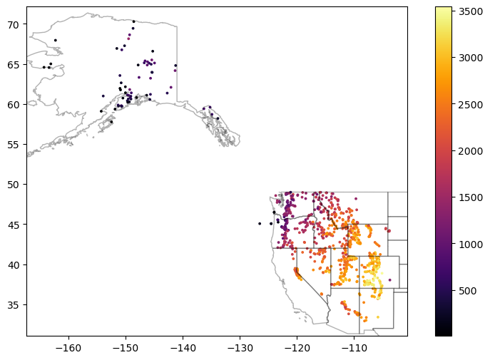
Create a scatterplot showing elevation values for all sites#
f, ax = plt.subplots(figsize=(10,6))
sites_gdf_all.plot(ax=ax, column='elevation_m', markersize=3, cmap='inferno', legend=True)
ax.autoscale(False)
states_gdf.plot(ax=ax, facecolor='none', edgecolor='k', alpha=0.3);
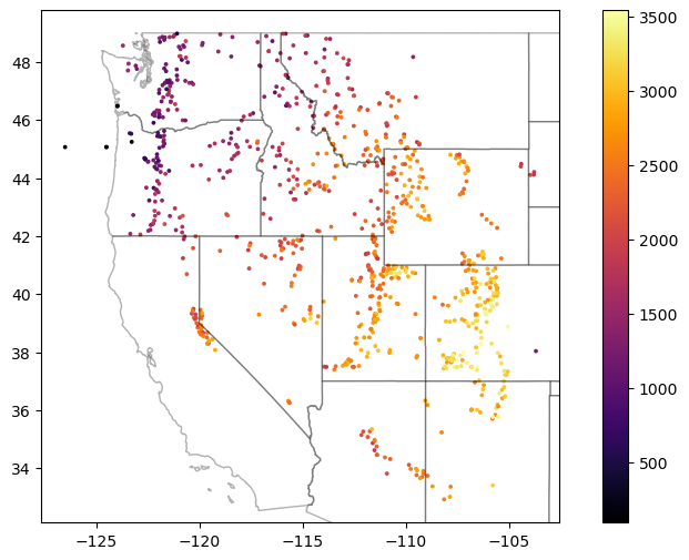
Exclude the Alaska (AK) points to isolate points over Western U.S.#
Can remove points where the site name contains ‘AK’ or can use a spatial filter (see GeoPandas cx indexer functionality)
Note the number of records
sites_gdf_all = sites_gdf_all[~(sites_gdf_all.index.str.contains('AK'))]
#xmin, xmax, ymin, ymax = [-126, 102, 30, 50]
#sites_gdf_all = sites_gdf_all.cx[xmin:xmax, ymin:ymax]
sites_gdf_all.shape
(865, 19)
Update scatterplot as sanity check#
Should look something like the Western U.S.
f, ax = plt.subplots(figsize=(10,6))
sites_gdf_all.plot(ax=ax, column='elevation_m', markersize=3, cmap='inferno', legend=True)
ax.autoscale(False)
states_gdf.plot(ax=ax, facecolor='none', edgecolor='k', alpha=0.3);
Export SNOTEL site GeoDataFrame as a geojson#
Maybe useful for later lab or other analysis
sites_fn = os.path.join(datadir, 'snotel_conus_sites.json')
if not os.path.exists(sites_fn):
    print('Writing out:', sites_fn)
    sites_gdf_all.to_file(sites_fn, driver='GeoJSON')
Part 2: Time series analysis for one station#
Now that we’ve identified sites of interest, let’s query the API to obtain the time series data for variables of interest (snow!).
#Interactive basemap - useful to select a site of interest
#sites_gdf_all.explore(column='elevation_m')
#Hart's Pass
#sitecode = 'SNOTEL:515_WA_SNTL'
#Paradise
sitecode = 'SNOTEL:679_WA_SNTL'
Query the server for information about this site#
Use the ulmo cuahsi
get_site_infomethod hereLots of output here, try to skim and get a sense of the different parameters and associated metadata
Note that there are many standard meteorological variables that can be downloaded for this site, in addition to the snow depth and snow water equivalent.
Careful about using some variables - documented bias in measurements
https://agupubs.onlinelibrary.wiley.com/doi/full/10.1002/2014GL062803
site_info = ulmo.cuahsi.wof.get_site_info(wsdlurl, sitecode)
#site_info
Inspect the returned information#
Note number of available variables in the time series data!
dict_keys = site_info['series'].keys()
dict_keys
dict_keys(['SNOTEL:BATT_D', 'SNOTEL:BATT_H', 'SNOTEL:PRCP_y', 'SNOTEL:PRCP_sm', 'SNOTEL:PRCP_m', 'SNOTEL:PRCP_wy', 'SNOTEL:PRCPSA_y', 'SNOTEL:PRCPSA_D', 'SNOTEL:PRCPSA_sm', 'SNOTEL:PRCPSA_m', 'SNOTEL:PRCPSA_wy', 'SNOTEL:PREC_sm', 'SNOTEL:PREC_m', 'SNOTEL:PREC_wy', 'SNOTEL:SNWD_D', 'SNOTEL:SNWD_sm', 'SNOTEL:SNWD_H', 'SNOTEL:SNWD_m', 'SNOTEL:TAVG_y', 'SNOTEL:TAVG_D', 'SNOTEL:TAVG_sm', 'SNOTEL:TAVG_m', 'SNOTEL:TAVG_wy', 'SNOTEL:TMAX_y', 'SNOTEL:TMAX_D', 'SNOTEL:TMAX_sm', 'SNOTEL:TMAX_m', 'SNOTEL:TMAX_wy', 'SNOTEL:TMIN_y', 'SNOTEL:TMIN_D', 'SNOTEL:TMIN_sm', 'SNOTEL:TMIN_m', 'SNOTEL:TMIN_wy', 'SNOTEL:TOBS_D', 'SNOTEL:TOBS_sm', 'SNOTEL:TOBS_H', 'SNOTEL:TOBS_m', 'SNOTEL:WTEQ_D', 'SNOTEL:WTEQ_sm', 'SNOTEL:WTEQ_H', 'SNOTEL:WTEQ_m'])
len(dict_keys)
41
Note on units:
_H = “hourly”
_D = “daily”
_sm, _m = “monthly”
_y = “yearly”
_wy = “water year”
Let’s consider the ‘SNOTEL:SNWD_D’ variable (Daily Snow Depth)#
Assign ‘SNOTEL:SNWD_D’ to a variable named
variablecodeGet some information about the variable using
get_variable_infomethodNote the units, nodata value, etc.
Note: The snow depth records are almost always shorter/noisier than the SWE records for SNOTEL sites
#Daily SWE
#variablecode = 'SNOTEL:WTEQ_D'
#Daily snow depth
variablecode = 'SNOTEL:SNWD_D'
#Hourly SWE
#variablecode = 'SNOTEL:WTEQ_H'
#Hourly snow depth
#variablecode = 'SNOTEL:SNWD_H'
ulmo.cuahsi.wof.get_variable_info(wsdlurl, variablecode)
{'value_type': 'Field Observation',
 'data_type': 'Continuous',
 'general_category': 'Soil',
 'sample_medium': 'Snow',
 'no_data_value': '-9999',
 'speciation': 'Not Applicable',
 'code': 'SNWD_D',
 'id': '176',
 'name': 'Snow depth',
 'vocabulary': 'SNOTEL',
 'time': {'is_regular': True,
  'interval': '1',
  'units': {'abbreviation': 'd',
   'code': '104',
   'name': 'day',
   'type': 'Time'}},
 'units': {'abbreviation': 'in',
  'code': '49',
  'name': 'international inch',
  'type': 'Length'}}
Define a function to fetch time series data#
Can define specific start and end dates, or get full record (default)
I’ve done this for you, but please review the comments and steps to see what is going on under the hood
You’ll probably have to do similar data wrangling for another project at some point in the future
today = pd.to_datetime("today")
today.strftime('%Y-%m-%d')
'2023-02-25'
#Get current datetime
today = pd.to_datetime("today").strftime('%Y-%m-%d')

def snotel_fetch(sitecode, variablecode='SNOTEL:SNWD_D', start_date='1950-10-01', end_date=today):
    #print(sitecode, variablecode, start_date, end_date)
    values_df = None
    try:
        #Request data from the server
        site_values = ulmo.cuahsi.wof.get_values(wsdlurl, sitecode, variablecode, start=start_date, end=end_date)
    except:
        print(f"Unable to fetch {variablecode} for {sitecode}")
    else:
        #Convert to a Pandas DataFrame
        values_df = pd.DataFrame.from_dict(site_values['values'])
        #Parse the datetime values to Pandas Timestamp objects
        values_df['datetime'] = pd.to_datetime(values_df['datetime'], utc=True)
        #Set the DataFrame index to the Timestamps
        values_df = values_df.set_index('datetime')
        #Convert values to float and replace -9999 nodata values with NaN
        values_df['value'] = pd.to_numeric(values_df['value']).replace(-9999, np.nan)
        #Remove any records flagged with lower quality
        values_df = values_df[values_df['quality_control_level_code'] == '1']

    return values_df
Use this function to get the full ‘SNOTEL:SNWD_D’ record for one station#
Inspect the results
We used a dummy start date of Jan 1, 1950. What is the actual the first date returned?
%%time
print(sitecode)
#values_df = snotel_fetch(sitecode, variablecode, start_date, end_date)
values_df = snotel_fetch(sitecode, variablecode)
SNOTEL:679_WA_SNTL
CPU times: user 686 ms, sys: 10.4 ms, total: 696 ms
Wall time: 3.21 s
values_df.head()
| value | qualifiers | censor_code | date_time_utc | method_id | method_code | source_code | quality_control_level_code | |
|---|---|---|---|---|---|---|---|---|
| datetime | ||||||||
| 2006-08-18 00:00:00+00:00 | 0.0 | E | nc | 2006-08-18T00:00:00 | 0 | 0 | 1 | 1 |
| 2006-08-19 00:00:00+00:00 | 0.0 | E | nc | 2006-08-19T00:00:00 | 0 | 0 | 1 | 1 |
| 2006-08-20 00:00:00+00:00 | 0.0 | E | nc | 2006-08-20T00:00:00 | 0 | 0 | 1 | 1 |
| 2006-08-21 00:00:00+00:00 | 0.0 | E | nc | 2006-08-21T00:00:00 | 0 | 0 | 1 | 1 |
| 2006-08-22 00:00:00+00:00 | 0.0 | E | nc | 2006-08-22T00:00:00 | 0 | 0 | 1 | 1 |
values_df.tail()
| value | qualifiers | censor_code | date_time_utc | method_id | method_code | source_code | quality_control_level_code | |
|---|---|---|---|---|---|---|---|---|
| datetime | ||||||||
| 2023-02-21 00:00:00+00:00 | 118.0 | V | nc | 2023-02-21T00:00:00 | 0 | 0 | 1 | 1 |
| 2023-02-22 00:00:00+00:00 | 123.0 | V | nc | 2023-02-22T00:00:00 | 0 | 0 | 1 | 1 |
| 2023-02-23 00:00:00+00:00 | NaN | NaN | nc | 2023-02-23T00:00:00 | 0 | 0 | 1 | 1 |
| 2023-02-24 00:00:00+00:00 | 124.0 | V | nc | 2023-02-24T00:00:00 | 0 | 0 | 1 | 1 |
| 2023-02-25 00:00:00+00:00 | 122.0 | V | nc | 2023-02-25T00:00:00 | 0 | 0 | 1 | 1 |
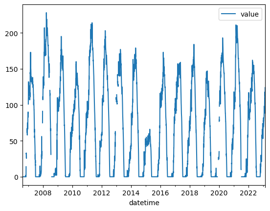
Create a quick plot to view the time series#
Take a moment to inspect the
valuecolumn, which is where theSNWD_Dvalues are storedSanity check thought question: What are the units again?
values_df.plot();
Write out the dataframe to disk#
Can use a number of different formats here, easiest to use a “pickle”: https://www.pythoncentral.io/how-to-pickle-unpickle-tutorial/
Define a unique filename for the dataset (e.g.,
pkl_fn='snotel_wa_snwd_d.pkl')Write the DataFrame to disk
pkl_fn = os.path.join(datadir, f"{variablecode.replace(':','-')}_{sitecode.split(':')[-1]}.pkl")
pkl_fn
'snotel_data/SNOTEL-SNWD_D_679_WA_SNTL.pkl'
print(f"Writing out: {pkl_fn}")
values_df.to_pickle(pkl_fn)
Writing out: snotel_data/SNOTEL-SNWD_D_679_WA_SNTL.pkl
Read it back in to check#
pd.read_pickle(pkl_fn)
| value | qualifiers | censor_code | date_time_utc | method_id | method_code | source_code | quality_control_level_code | |
|---|---|---|---|---|---|---|---|---|
| datetime | ||||||||
| 2006-08-18 00:00:00+00:00 | 0.0 | E | nc | 2006-08-18T00:00:00 | 0 | 0 | 1 | 1 |
| 2006-08-19 00:00:00+00:00 | 0.0 | E | nc | 2006-08-19T00:00:00 | 0 | 0 | 1 | 1 |
| 2006-08-20 00:00:00+00:00 | 0.0 | E | nc | 2006-08-20T00:00:00 | 0 | 0 | 1 | 1 |
| 2006-08-21 00:00:00+00:00 | 0.0 | E | nc | 2006-08-21T00:00:00 | 0 | 0 | 1 | 1 |
| 2006-08-22 00:00:00+00:00 | 0.0 | E | nc | 2006-08-22T00:00:00 | 0 | 0 | 1 | 1 |
| ... | ... | ... | ... | ... | ... | ... | ... | ... |
| 2023-02-21 00:00:00+00:00 | 118.0 | V | nc | 2023-02-21T00:00:00 | 0 | 0 | 1 | 1 |
| 2023-02-22 00:00:00+00:00 | 123.0 | V | nc | 2023-02-22T00:00:00 | 0 | 0 | 1 | 1 |
| 2023-02-23 00:00:00+00:00 | NaN | NaN | nc | 2023-02-23T00:00:00 | 0 | 0 | 1 | 1 |
| 2023-02-24 00:00:00+00:00 | 124.0 | V | nc | 2023-02-24T00:00:00 | 0 | 0 | 1 | 1 |
| 2023-02-25 00:00:00+00:00 | 122.0 | V | nc | 2023-02-25T00:00:00 | 0 | 0 | 1 | 1 |
6036 rows × 8 columns
Part 3: Retrieve time series records for All SNOTEL Sites#
Now that we’ve explored one site, let’s look at them all!
Probably going to be some interesting spatial/temporal variability in these metrics
Notes:#
I’ve providing the following code to do this for you. Please review so you understand what’s going on:
Loop through all sites names in the sites GeoDataFrame and run the above
snotel_fetchfunctionStore output in a dictionary
Convert the dictionary to a Pandas Dataframe
Write final output to disk
Note that this could take some time to run for all SNOTEL sites (~10-40 min, depending on server load)
Progress will be printed out incrementally
While you wait, explore some of the above links, or review remainder of lab
Several sites may return an error (e.g.,
<suds.sax.document.Document object at 0x7f0813040730>)Fortunately, this is handled by the
try-exceptblock in thesnotel_fetchfunction aboveThis warning could arise for a number of reasons:
The site doesn’t have an ultrasonic snow depth sensor: https://doi.org/10.1175/2007JTECHA947.1
The site was decomissioned or never produced valid data
The data are not available on the CUAHSI server
There was an issue connecting with the CUAHSI server
Most likely the first issue. Some of these sites should have valid records for SWE, but not SD
#Fetch desired SNOTEL data for all sites in the provided GeoDataFrame
def snotel_fetch_multisite(gdf, variablecode, pkl_fn):
    if os.path.exists(pkl_fn):
        snwd_df = pd.read_pickle(pkl_fn)
    else:
        #Define an empty dictionary to store returns for each site
        value_dict = {}
        #Loop through each site and add record to dictionary
        for i, sitecode in enumerate(gdf.index):
            print('%i of %i sites: %s' % (i+1, len(gdf.index), sitecode))
            #out = snotel_fetch(sitecode, variablecode, start_date, end_date)
            out = snotel_fetch(sitecode, variablecode)
            if out is not None:
                value_dict[sitecode] = out['value']

        #Convert the dictionary to a DataFrame, automatically handles different datetime ranges (nice!)
        snwd_df = pd.DataFrame.from_dict(value_dict)
        #Write out
        print(f"Writing out: {pkl_fn}")
        snwd_df.to_pickle(pkl_fn)
    return snwd_df
Prepare SNWD_D for all CONUS sites#
%%time
variablecode = 'SNOTEL:SNWD_D'
pkl_fn = os.path.join(datadir, f"{variablecode.replace(':','-')}_CONUS_all.pkl")

snwd_df = snotel_fetch_multisite(sites_gdf_all, variablecode, pkl_fn)
CPU times: user 196 µs, sys: 96.4 ms, total: 96.6 ms
Wall time: 96.3 ms
Prepare WTEQ_D for all WA sites#
We will use this for Week09 demo
#Isolate WA sites
wa_idx = sites_gdf_all.index.str.contains('WA')
sites_gdf_wa = sites_gdf_all[wa_idx]
sites_gdf_wa.shape
(84, 19)
%%time
variablecode = 'SNOTEL:WTEQ_D'
pkl_fn = os.path.join(datadir, f"{variablecode.replace(':','-')}_WA.pkl")

wteq_df = snotel_fetch_multisite(sites_gdf_wa, variablecode, pkl_fn)
CPU times: user 293 µs, sys: 13.4 ms, total: 13.7 ms
Wall time: 11.2 ms
Inspect the DataFrame#
Note structure, number of timestamps, NaNs
What is the date of the first snow depth measurement in the network?
Note that the water equivalent (WTEQ_D) measurements from snow pillows extend much farther back in time, back to the early 1980s, before the ultrasonic snow depth instruments were incorporated across the network. These are better to use for long-term studies.
snwd_df.shape
(14025, 806)
snwd_df.head()
| SNOTEL:301_CA_SNTL | SNOTEL:907_UT_SNTL | SNOTEL:916_MT_SNTL | SNOTEL:908_WA_SNTL | SNOTEL:302_OR_SNTL | SNOTEL:1000_OR_SNTL | SNOTEL:303_CO_SNTL | SNOTEL:1030_CO_SNTL | SNOTEL:304_OR_SNTL | SNOTEL:306_ID_SNTL | ... | SNOTEL:872_WY_SNTL | SNOTEL:873_OR_SNTL | SNOTEL:874_CO_SNTL | SNOTEL:875_WY_SNTL | SNOTEL:876_MT_SNTL | SNOTEL:877_AZ_SNTL | SNOTEL:1228_UT_SNTL | SNOTEL:1197_UT_SNTL | SNOTEL:878_WY_SNTL | SNOTEL:1033_CO_SNTL | |
|---|---|---|---|---|---|---|---|---|---|---|---|---|---|---|---|---|---|---|---|---|---|
| datetime | |||||||||||||||||||||
| 1984-10-01 00:00:00+00:00 | NaN | NaN | NaN | NaN | NaN | NaN | NaN | NaN | NaN | NaN | ... | NaN | NaN | NaN | NaN | NaN | NaN | NaN | NaN | NaN | NaN |
| 1984-10-02 00:00:00+00:00 | NaN | NaN | NaN | NaN | NaN | NaN | NaN | NaN | NaN | NaN | ... | NaN | NaN | NaN | NaN | NaN | NaN | NaN | NaN | NaN | NaN |
| 1984-10-03 00:00:00+00:00 | NaN | NaN | NaN | NaN | NaN | NaN | NaN | NaN | NaN | NaN | ... | NaN | NaN | NaN | NaN | NaN | NaN | NaN | NaN | NaN | NaN |
| 1984-10-04 00:00:00+00:00 | NaN | NaN | NaN | NaN | NaN | NaN | NaN | NaN | NaN | NaN | ... | NaN | NaN | NaN | NaN | NaN | NaN | NaN | NaN | NaN | NaN |
| 1984-10-05 00:00:00+00:00 | NaN | NaN | NaN | NaN | NaN | NaN | NaN | NaN | NaN | NaN | ... | NaN | NaN | NaN | NaN | NaN | NaN | NaN | NaN | NaN | NaN |
5 rows × 806 columns
snwd_df.tail()
| SNOTEL:301_CA_SNTL | SNOTEL:907_UT_SNTL | SNOTEL:916_MT_SNTL | SNOTEL:908_WA_SNTL | SNOTEL:302_OR_SNTL | SNOTEL:1000_OR_SNTL | SNOTEL:303_CO_SNTL | SNOTEL:1030_CO_SNTL | SNOTEL:304_OR_SNTL | SNOTEL:306_ID_SNTL | ... | SNOTEL:872_WY_SNTL | SNOTEL:873_OR_SNTL | SNOTEL:874_CO_SNTL | SNOTEL:875_WY_SNTL | SNOTEL:876_MT_SNTL | SNOTEL:877_AZ_SNTL | SNOTEL:1228_UT_SNTL | SNOTEL:1197_UT_SNTL | SNOTEL:878_WY_SNTL | SNOTEL:1033_CO_SNTL | |
|---|---|---|---|---|---|---|---|---|---|---|---|---|---|---|---|---|---|---|---|---|---|
| datetime | |||||||||||||||||||||
| 2023-02-19 00:00:00+00:00 | 42.0 | 33.0 | 48.0 | 78.0 | 55.0 | 76.0 | 8.0 | 60.0 | 44.0 | 68.0 | ... | 27.0 | 48.0 | 88.0 | 29.0 | 25.0 | 26.0 | 39.0 | 37.0 | 35.0 | 63.0 |
| 2023-02-20 00:00:00+00:00 | 41.0 | 32.0 | 47.0 | 84.0 | 56.0 | 75.0 | 8.0 | 62.0 | 44.0 | 70.0 | ... | 28.0 | 49.0 | 88.0 | 33.0 | 26.0 | 24.0 | 39.0 | 36.0 | 37.0 | 68.0 |
| 2023-02-21 00:00:00+00:00 | 40.0 | 31.0 | 46.0 | 86.0 | 55.0 | 73.0 | 10.0 | 61.0 | 43.0 | 71.0 | ... | 29.0 | 48.0 | 86.0 | 42.0 | 33.0 | 21.0 | 39.0 | 35.0 | 42.0 | 68.0 |
| 2023-02-22 00:00:00+00:00 | 40.0 | 32.0 | 53.0 | NaN | 56.0 | 83.0 | 6.0 | NaN | 51.0 | 76.0 | ... | 39.0 | 52.0 | 86.0 | 45.0 | 35.0 | 19.0 | 44.0 | 34.0 | 46.0 | 70.0 |
| 2023-02-23 00:00:00+00:00 | 44.0 | 38.0 | 52.0 | 91.0 | 56.0 | 90.0 | 8.0 | 67.0 | 52.0 | 78.0 | ... | NaN | 57.0 | 98.0 | 44.0 | 33.0 | 23.0 | 45.0 | 41.0 | 45.0 | 73.0 |
5 rows × 806 columns
snwd_df.describe()
| SNOTEL:301_CA_SNTL | SNOTEL:907_UT_SNTL | SNOTEL:916_MT_SNTL | SNOTEL:908_WA_SNTL | SNOTEL:302_OR_SNTL | SNOTEL:1000_OR_SNTL | SNOTEL:303_CO_SNTL | SNOTEL:1030_CO_SNTL | SNOTEL:304_OR_SNTL | SNOTEL:306_ID_SNTL | ... | SNOTEL:872_WY_SNTL | SNOTEL:873_OR_SNTL | SNOTEL:874_CO_SNTL | SNOTEL:875_WY_SNTL | SNOTEL:876_MT_SNTL | SNOTEL:877_AZ_SNTL | SNOTEL:1228_UT_SNTL | SNOTEL:1197_UT_SNTL | SNOTEL:878_WY_SNTL | SNOTEL:1033_CO_SNTL | |
|---|---|---|---|---|---|---|---|---|---|---|---|---|---|---|---|---|---|---|---|---|---|
| count | 8971.000000 | 8909.000000 | 9660.000000 | 6833.000000 | 7954.000000 | 8193.000000 | 8365.000000 | 7139.000000 | 7197.000000 | 9711.000000 | ... | 6349.000000 | 6461.000000 | 9104.000000 | 7864.000000 | 7533.000000 | 6920.000000 | 3863.000000 | 3879.000000 | 8272.000000 | 7284.000000 |
| mean | 9.815851 | 7.407790 | 24.913458 | 36.359579 | 27.014332 | 35.334798 | 5.964136 | 29.431013 | 15.439489 | 32.198126 | ... | 9.114506 | 15.036372 | 34.276911 | 11.033698 | 10.453339 | 3.697688 | 10.476831 | 8.383346 | 18.256770 | 26.014690 |
| std | 14.651453 | 12.660844 | 23.422584 | 42.755263 | 26.955982 | 40.036953 | 9.399264 | 27.698495 | 19.887877 | 35.128416 | ... | 11.477779 | 19.419041 | 36.237121 | 14.216598 | 12.869854 | 7.669382 | 14.125755 | 11.750906 | 20.047268 | 29.159213 |
| min | 0.000000 | 0.000000 | 0.000000 | 0.000000 | 0.000000 | 0.000000 | 0.000000 | 0.000000 | 0.000000 | 0.000000 | ... | 0.000000 | 0.000000 | 0.000000 | 0.000000 | 0.000000 | 0.000000 | 0.000000 | 0.000000 | 0.000000 | 0.000000 |
| 25% | 0.000000 | 0.000000 | 0.000000 | 0.000000 | 0.000000 | 0.000000 | 0.000000 | 0.000000 | 0.000000 | 0.000000 | ... | 0.000000 | 0.000000 | 0.000000 | 0.000000 | 0.000000 | 0.000000 | 0.000000 | 0.000000 | 0.000000 | 0.000000 |
| 50% | 0.000000 | 0.000000 | 22.000000 | 17.000000 | 21.000000 | 20.000000 | 0.000000 | 24.000000 | 0.000000 | 19.000000 | ... | 3.000000 | 0.000000 | 25.000000 | 1.000000 | 4.000000 | 0.000000 | 0.000000 | 0.000000 | 10.000000 | 13.000000 |
| 75% | 18.000000 | 12.000000 | 44.000000 | 69.000000 | 48.000000 | 67.000000 | 9.000000 | 55.000000 | 32.000000 | 60.000000 | ... | 17.000000 | 31.000000 | 63.000000 | 22.000000 | 20.000000 | 3.000000 | 22.000000 | 17.000000 | 34.000000 | 51.000000 |
| max | 66.000000 | 70.000000 | 95.000000 | 175.000000 | 107.000000 | 162.000000 | 53.000000 | 106.000000 | 76.000000 | 144.000000 | ... | 139.000000 | 75.000000 | 198.000000 | 64.000000 | 61.000000 | 56.000000 | 60.000000 | 55.000000 | 79.000000 | 111.000000 |
8 rows × 806 columns