09 Exercises 1: Intro and Global Temperature Analysis
Contents
09 Exercises 1: Intro and Global Temperature Analysis#
UW Geospatial Data Analysis
CEE467/CEWA567
David Shean
Objectives#
Introduce xarray data model for N-d array analysis
Practice basic N-d array slicing, grouping and aggregation
Explore global and local climate reanalysis data
import os
from glob import glob
import numpy as np
import xarray as xr
import pandas as pd
import geopandas as gpd
import cartopy.crs as ccrs
import matplotlib.pyplot as plt
import holoviews as hv
Part 1: Global climatology#
Monthly temperature from 1979-2021#
Two datasets are provided:
Climatology - long-term mean monthly values ofrom 1979-2021 (12 grids)
Anomaly - monthly difference from long-term monthly mean (505 grids from 1979-2021)
See here for more details: https://cds.climate.copernicus.eu/cdsapp#!/dataset/ecv-for-climate-change?tab=overview
%pwd
'/home/jovyan/src/gda_course_2023_solutions/modules/09_NDarrays_xarray_ERA5'
Open the processed global monthly temperature anomaly and climatology NetCDF files#
See relevant doc on opening and writing files: http://xarray.pydata.org/en/stable/io.html
Note that processing and saving the anomalies could take some time, as you’re reading in 480 files and saving a large nc file
Take a moment to review the steps in the
grib2ncfunction of the download notebook, and review the io doc for xarrayNote the
open_datasetandconcatfunctions
era5_datadir = '/home/jovyan/jupyterbook/book/modules/09_NDarrays_xarray_ERA5/era5_data'
!ls -lh $era5_datadir
total 3.9G
-rw-rw-r-- 1 jovyan users 2.0G Feb 27 00:47 1month_anomaly_Global_ea_2t.nc
-rw-rw-r-- 1 jovyan users  48M Feb 27 00:47 climatology_0.25g_ea_2t.nc
-rw-rw-r-- 1 jovyan users 1.9G Feb 27 00:47 WA_ERA5-Land_hourly_1950-2022_6hr.nc
t_clim_fn = os.path.join(era5_datadir, 'climatology_0.25g_ea_2t.nc')
t_clim_ds = xr.open_dataset(t_clim_fn)
t_anom_fn = os.path.join(era5_datadir, '1month_anomaly_Global_ea_2t.nc')
t_anom_ds = xr.open_dataset(t_anom_fn, chunks='auto')
Inspect the DataSets#
Discuss with your neighbor
Review the output when you just type the DataSet name (similar to output from the
info()method)Note the number of time entries in each DataSet
What are the min and max longitude, min and max latitude
Note: The timestamp listed in the climatology dataset for each month is arbitrarily listed as 2018 (e.g., ‘2018-01-01’)
Remember these are mean values for each month of the year (12 total) across the entire 1979-2021 period
print info for the ‘t2m’ DataArray (temperature 2 m above ground)
t_clim_ds
<xarray.Dataset>
Dimensions:    (time: 12, latitude: 721, longitude: 1440)
Coordinates:
  * time       (time) datetime64[ns] 1981-01-01 1981-02-01 ... 1981-12-01
  * latitude   (latitude) float64 90.0 89.75 89.5 89.25 ... -89.5 -89.75 -90.0
  * longitude  (longitude) float64 0.0 0.25 0.5 0.75 ... 359.0 359.2 359.5 359.8
Data variables:
    t2m        (time, latitude, longitude) float32 ...
Attributes:
    GRIB_edition:            1
    GRIB_centre:             ecmf
    GRIB_centreDescription:  European Centre for Medium-Range Weather Forecasts
    GRIB_subCentre:          0
    Conventions:             CF-1.7
    institution:             European Centre for Medium-Range Weather Forecasts
history: 2022-02-28T07:58 GRIB to CDM+CF via cfgrib-0.9.1...t_anom_ds
<xarray.Dataset>
Dimensions: (time: 517, latitude: 721, longitude: 1440)
Coordinates:
* time (time) datetime64[ns] 1979-01-01 1979-02-01 ... 2022-01-01
* latitude (latitude) float64 90.0 89.75 89.5 89.25 ... -89.5 -89.75 -90.0
* longitude (longitude) float64 0.0 0.25 0.5 0.75 ... 359.0 359.2 359.5 359.8
Data variables:
t2m (time, latitude, longitude) float32 dask.array<chunksize=(205, 286, 571), meta=np.ndarray>
Attributes:
GRIB_edition: 1
GRIB_centre: ecmf
GRIB_centreDescription: European Centre for Medium-Range Weather Forecasts
GRIB_subCentre: 0
Conventions: CF-1.7
institution: European Centre for Medium-Range Weather Forecasts
history: 2022-02-28T07:59 GRIB to CDM+CF via cfgrib-0.9.1...Convert the temperature values from K to C for the climatology dataset#
Note: don’t need to do this for anomalies, as they are relative values, not absolute
These operations are done on the DataArray level (not the top-level DataSet object level), so you’ll need to modify
t_clim_ds['t2m']You can use
-=syntax hereOr, update the
t_clim_ds['t2m'].values
Make sure you also update the units metadata attribute
The units used by xarray are stored in the t_clim_ds[‘t2m’].attrs dictionary
There is also a GRIB units variable, but this is holdover from the grib to xarray conversion
Sanity check values
#Student Exercise
#Student Exercise
{'GRIB_paramId': 167,
'GRIB_dataType': 'an',
'GRIB_numberOfPoints': 1038240,
'GRIB_typeOfLevel': 'surface',
'GRIB_stepUnits': 1,
'GRIB_stepType': 'avgua',
'GRIB_gridType': 'regular_ll',
'GRIB_NV': 0,
'GRIB_Nx': 1440,
'GRIB_Ny': 721,
'GRIB_cfName': 'unknown',
'GRIB_cfVarName': 't2m',
'GRIB_gridDefinitionDescription': 'Latitude/Longitude Grid',
'GRIB_iDirectionIncrementInDegrees': 0.25,
'GRIB_iScansNegatively': 0,
'GRIB_jDirectionIncrementInDegrees': 0.25,
'GRIB_jPointsAreConsecutive': 0,
'GRIB_jScansPositively': 0,
'GRIB_latitudeOfFirstGridPointInDegrees': 90.0,
'GRIB_latitudeOfLastGridPointInDegrees': -90.0,
'GRIB_longitudeOfFirstGridPointInDegrees': 0.0,
'GRIB_longitudeOfLastGridPointInDegrees': 359.75,
'GRIB_missingValue': 9999,
'GRIB_name': '2 metre temperature',
'GRIB_shortName': '2t',
'GRIB_totalNumber': 0,
'GRIB_units': 'C',
'long_name': '2 metre temperature',
'units': 'C',
'standard_name': 'unknown',
'coordinates': 'number time step surface latitude longitude valid_time'}
Set the longitude values to be (-180 to 180) instead of (0 to 360)#
Could also store as new set of coordinates called
longitude_180or something
def ds_swaplon(ds):
return ds.assign_coords(longitude=(((ds.longitude + 180) % 360) - 180)).sortby('longitude')
t_clim_ds = ds_swaplon(t_clim_ds)
t_anom_ds = ds_swaplon(t_anom_ds)
t_clim_ds.longitude
<xarray.DataArray 'longitude' (longitude: 1440)> array([-180. , -179.75, -179.5 , ..., 179.25, 179.5 , 179.75]) Coordinates: * longitude (longitude) float64 -180.0 -179.8 -179.5 ... 179.2 179.5 179.8
Isolate the data for the month of August and plot#
Review different strategies for selection here: http://xarray.pydata.org/en/stable/indexing.html
Try the
iselmethod with dimension name and integer index (e.g.,time=7)Try the
selmethod with dimension name and label (e.g.,time='2016-08-01', though the year may be different in your dataset)Note: the xarray convenience
plot.imshow()is much more efficient for regular grids than the defaultplot(), which usescontourfto interpolate values not on a regular gridSee the note here: https://xarray-test.readthedocs.io/en/latest/plotting.html#two-dimensions
Try the
robust=Trueoption
#See time dimension index
t_clim_ds.time
<xarray.DataArray 'time' (time: 12)>
array(['1981-01-01T00:00:00.000000000', '1981-02-01T00:00:00.000000000',
       '1981-03-01T00:00:00.000000000', '1981-04-01T00:00:00.000000000',
       '1981-05-01T00:00:00.000000000', '1981-06-01T00:00:00.000000000',
       '1981-07-01T00:00:00.000000000', '1981-08-01T00:00:00.000000000',
       '1981-09-01T00:00:00.000000000', '1981-10-01T00:00:00.000000000',
       '1981-11-01T00:00:00.000000000', '1981-12-01T00:00:00.000000000'],
      dtype='datetime64[ns]')
Coordinates:
* time (time) datetime64[ns] 1981-01-01 1981-02-01 ... 1981-12-01
Attributes:
long_name: initial time of forecast
standard_name: forecast_reference_time#Student Exercise
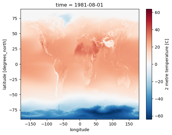
Create a plot for August, overlaying coastlines with cartopy#
Use a simple PlateCaree() projection as in example here:
Once you have your axes setup, you should be able to plot with xarray easily (pass the axes object to plot() function:
http://xarray.pydata.org/en/stable/plotting.html#maps
Don’t use a discrete color ramp as in some of the examples, use a continuous linear color ramp, as in the facet plot.
Note how 2-m temperature varies with elevation (e.g., see the Tibetan Plateau)
f = plt.figure()
ax = plt.axes(projection=ccrs.PlateCarree())
ax.coastlines()
ts = '1981-08-01'
t_clim_ds['t2m'].sel(time=ts).plot.imshow(ax=ax, robust=True);
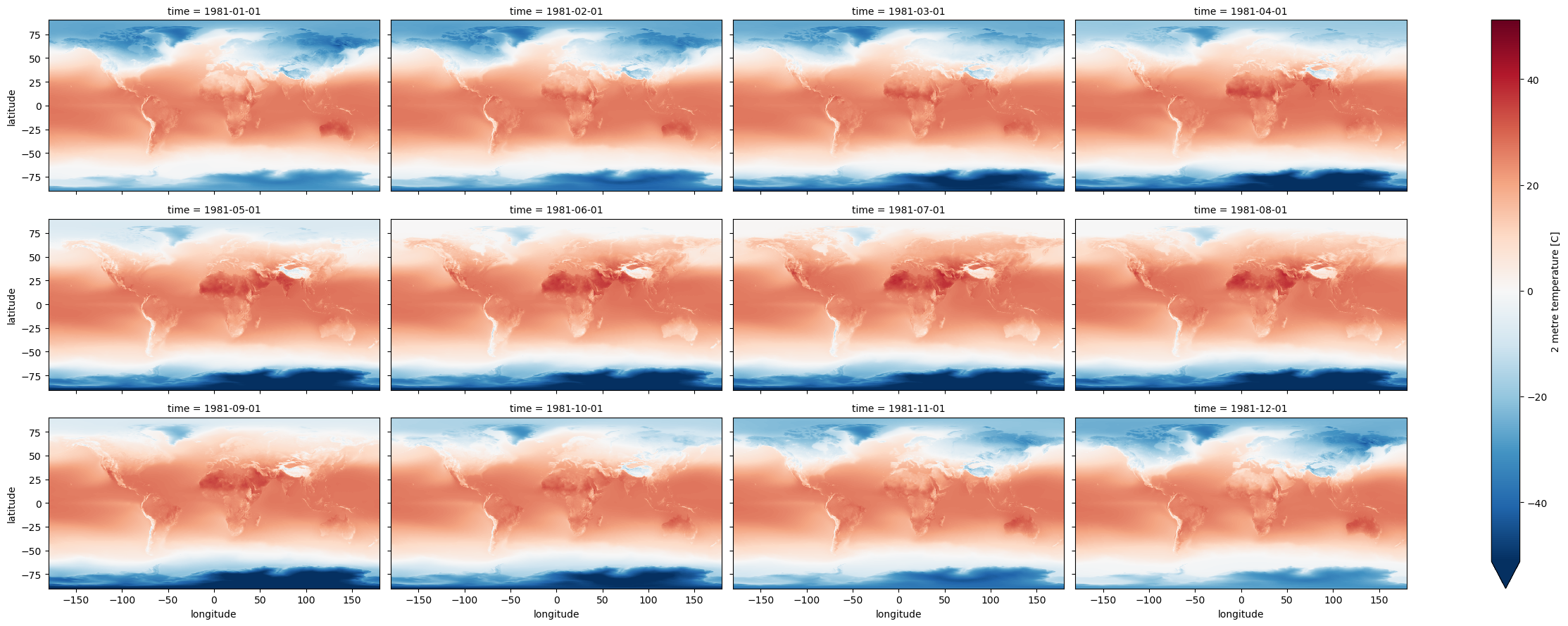
Create a Facet plot showing temperature grids for each month in the climatology DataSet#
Note that these plots can be memory hungry, and if you have other kernels running, this could fill RAM and cause kernel to stop
Could try isolating a smaller area to test (see slicing) then running on full dataset when satisfied
Make sure your units are correct in the colorbar
Note that xarray uses a different definition of
aspectthan matplotlibhttps://docs.xarray.dev/en/stable/user-guide/plotting.html#controlling-the-figure-size
Since we have 360° of longitude and 180° of latitude, an aspect of 2 should work well here
While they may look similar, each panel is slightly different
Take a moment to admire this, look at seasonal cycles
#Student Exercise
Use Holoviz for interactive plotting#
Multiple plotting backends can be used with xarray
We previously used Seaborn, and folium/ipyleaflet for interactive maps
Still under development, but
hvplotis flexible and powerful:
import hvplot.xarray
Create interactive plot with hvplot()#
Note how coordinates and values are interactively displayed as you move your cursor over the plot
Experiment with time slider on right side
Experiment with zoom/pan capability
#t_clim_ds['t2m'].hvplot(x='longitude',y='latitude', cmap='RdBu_r', clim=(-50,50))
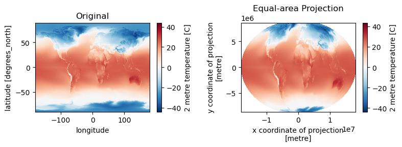
Reprojecting with rioxarray#
Those visualizations are nice, but we have a problem for further analysis…
The netcdf files have equally spaced grid points every 0.25° of latitude and longitude, which means we are oversampling in the polar regions
Think back to Lab04 about the true distance covered by 0.25° degree of longitude near the pole (close to 0 m) vs 0.25° of longitude near the equator (~28 km)
The default Plate Carrée “projection” (cylindrical equidistant) for lat/lon data is fine for quick visualization, but it distorts area, especially in the polar regions
If we compute mean or other statistics without accounting for this, our results will be biased, incorrectly weigthing the polar regions
Fortunately, we can use
rioxarrayto quickly reproject into an equal-area projection for these calculationsFirst need to assigning a crs to the xarray dataset
Can then use
xds.rio.reproject()https://corteva.github.io/rioxarray/stable/examples/reproject.html
Caveat: The better way to do this would be to use the original Gaussian grid from the model, but since we have the netCDF data on regular grid, let’s just work with those
import rioxarray
#Set CRS of the original xarray Datasets
t_clim_ds.rio.write_crs('EPSG:4326', inplace=True);
t_anom_ds.rio.write_crs('EPSG:4326', inplace=True);
#print(t_clim_ds.spatial_ref)
#Cylindrical equal area
ea_proj = '+proj=cea +lat_ts=45'
#Equal Earth (not working correctly)
ea_proj = '+proj=eqearth'
#Mollweide
ea_proj = '+proj=moll'
#ea_proj = 'EPSG:6933'
#Reproject and store output
t_clim_ds_proj = t_clim_ds['t2m'].rio.reproject(ea_proj, resampling=3)
#Reverse projection
#Note: output only spans -81 to 81°, not original -90° to 90°, need to revisit
#t_clim_ds_proj.rio.reproject('EPSG:4326')['y'].min()
#t_clim_ds_proj.rio.reproject('EPSG:4326', resampling=3).isel(time=0).plot.imshow()
f, axa = plt.subplots(1,2, figsize=(8,3))
t_clim_ds['t2m'].isel(time=0).plot.imshow(ax=axa[0])
axa[0].set_title('Original')
t_clim_ds_proj.isel(time=0).plot.imshow(ax=axa[1])
axa[1].set_title('Equal-area Projection')
plt.tight_layout()
Compare mean values for the two projections#
print("Original global mean T:", t_clim_ds['t2m'].mean().values)
print("Equal-area projection global mean T:", t_clim_ds_proj.mean().values)
Original global mean T: 5.2075896
Equal-area projection global mean T: 14.664276
Much closer to expected value of 13.9° for 20th Century (https://www.ncei.noaa.gov/access/monitoring/monthly-report/global/)
Remember that our dataset is for 1979-2022 period, so we actually expect it to be slightly warmer than the average for the 1900-2000 period
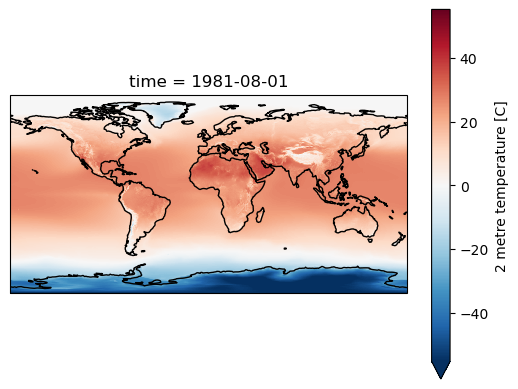
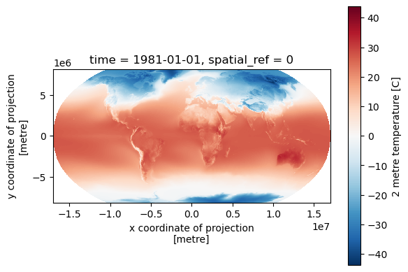
Visualization using Robinson Projection#
This is a good compromise for global plots
But it is not equal area
Equal Earth is a better option: https://proj.org/operations/projections/eqearth.html
Unfortunately, there is a bug in rioxarray/PROJ and this is not working correctly for this dataset
f, ax = plt.subplots()
t_clim_ds['t2m'].isel(time=0).rio.reproject('+proj=robin', resampling=3).plot.imshow(ax=ax)
ax.set_aspect('equal')
Define variables for remainder of lab#
#Using original EPSG:4326 lat/lon
#t_clim_da = t_clim_ds['t2m']
#xdim = 'longitude'
#ydim = 'latitude'
#Using cylindrical equal area projection for analysis
t_clim_da = t_clim_ds_proj
xdim = 'x'
ydim = 'y'
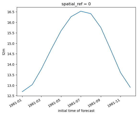
Create line plot of global monthly temperature#
Compute the mean of the reprojected climatology t2m DataArray across the spatial dimensions (both x and y)
Remember to pass the appropriate
dim=(...)tomean()so xarray knows over which dimensions to compute the mean!)
#Not this! Gives a single value for full array
#t_clim_da.mean()
#Student Exercise
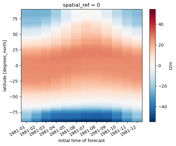
Create 2D plot showing mean temperature vs. latitude (averaged over all longitudes)#
#Student Exercise
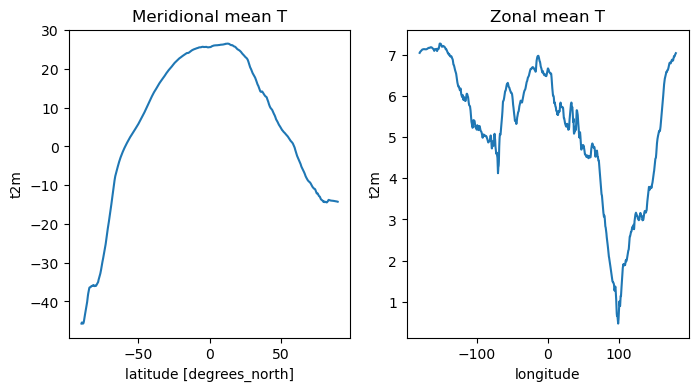
Create line plots of mean zonal and meridional temperature#
Hint: specify a tuple of appropriate dimensions for the
dimkeyword when computingmean()Above we used
dim=('latitude', 'longitude')to average all latitudes and longitudes, plotting the resulting values over timeNow in the zonal mean case, we want to average for all latitudes and times, plotting resulting values vs. longitude
Create as figure with two subplots: meridional mean T and zonal mean T
Add titles accordingly
#Student Exercise
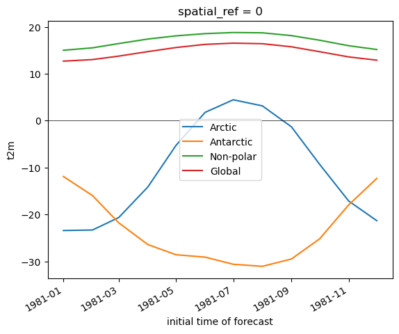
Create a plot showing monthly mean temperature for the Arctic and Antarctic#
See location indexing here: http://xarray.pydata.org/en/stable/indexing.html#assigning-values-with-indexing
One approach:
Create boolean index arrays for
t_clim_ds['latitude']coordinate for relevant latitude rangesUse Arctic circle and Antarctic circle as a threshold
Use the index array with xarray
wheremethod on thet_clim_ds['t2m']DataArrayMake sure to use
drop=Trueto avoid unnecessarily storing lots of nan values in memory
Compute the mean across all returned lat/lon grid cells
Note the magnitude and phase of the seasonal temperature varability at the opposite poles
polar_lat = 66.5 #degrees
Convert polar circle latitude to y-coordinate for equal area projection#
#Compute y coordinate of polar circle latitude
from pyproj import CRS, Transformer
transformer = Transformer.from_crs(CRS.from_epsg(4326), CRS.from_proj4(ea_proj))
polar_y = transformer.transform(polar_lat, 0)[-1]
polar_y
7474236.788842151
if ydim == 'latitude':
    polar_y = polar_lat
polar_y
7474236.788842151
arctic_idx = (t_clim_da[ydim] >= polar_y)
antarctic_idx = (t_clim_da[ydim] <= -polar_y)
nonpolar_idx = (t_clim_da[ydim] < polar_y) & (t_clim_da[ydim] > -polar_y)
#Sanity check
#arctic_idx[::10]
#antarctic_idx[::10]
#nonpolar_idx[::10]
kwargs = dict(cmap='RdBu_r', vmin=-50, vmax=50)
#Student Exercise
#Student Exercise
Extra Credit: Repeat the above analysis, isolating land and ocean classes#
Hint: can use
rioxarrayfor clipping using a GeoDataFrame or geometry
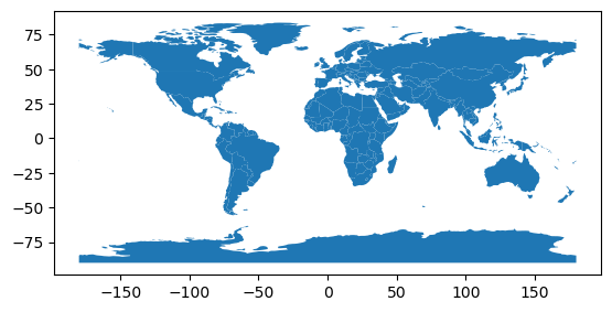
Open the world polygons#
world = gpd.read_file(gpd.datasets.get_path('naturalearth_lowres'))
#Hack to set to latest PROJ syntax, instead of 'init'
world.crs = 'EPSG:4326'
world.plot();
#world.to_crs(ea_proj).plot();
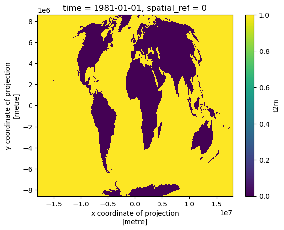
Use rioxarray clip function#
Code and documentation is still under development, but you can read more here:
#Mask values over ocean
t_clim_ds_land = t_clim_da.rio.clip(world.to_crs(t_clim_da.rio.crs).geometry, crs=t_clim_da.rio.crs, drop=False)
#Invert to mask values over land
t_clim_ds_ocean = t_clim_da.rio.clip(world.to_crs(t_clim_da.rio.crs).geometry, crs=t_clim_da.rio.crs, drop=False, invert=True)
#Preview land mask
t_clim_ds_land.isel(time=0).isnull().plot.imshow();
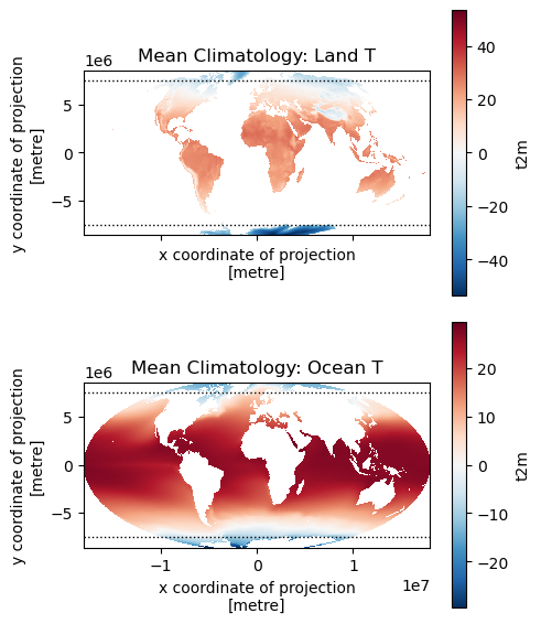
Create maps for land and ocean T#
f, axa = plt.subplots(2,1, sharex=True, sharey=True, figsize=(5,6))
t_clim_ds_land.mean(dim='time').plot(ax=axa[0], cmap='RdBu_r', clim=(-50,50))
t_clim_ds_ocean.mean(dim='time').plot(ax=axa[1], cmap='RdBu_r', clim=(-50,50))
axa[0].set_title('Mean Climatology: Land T')
axa[1].set_title('Mean Climatology: Ocean T')
kwargs = dict(color='k', lw=1.0, ls=':')
for ax in axa:
    ax.axhline(polar_y, **kwargs)
    ax.axhline(-polar_y, **kwargs)
    ax.set_aspect('equal')
plt.tight_layout()
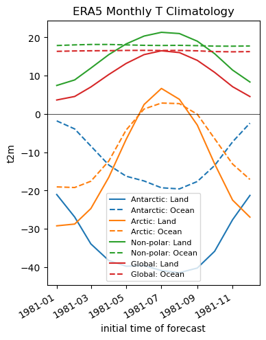
Create line plots for land and ocean T#
f, ax = plt.subplots(figsize=(4,5))
t_clim_ds_land.where(antarctic_idx, drop=True).mean(dim=(xdim, ydim)).plot(ax=ax, color='C0', ls='-', label='Antarctic: Land')
t_clim_ds_ocean.where(antarctic_idx, drop=True).mean(dim=(xdim, ydim)).plot(ax=ax, color='C0', ls='--', label='Antarctic: Ocean')
t_clim_ds_land.where(arctic_idx, drop=True).mean(dim=(xdim, ydim)).plot(ax=ax, color='C1', ls='-', label='Arctic: Land')
t_clim_ds_ocean.where(arctic_idx, drop=True).mean(dim=(xdim, ydim)).plot(ax=ax, color='C1', ls='--', label='Arctic: Ocean')
t_clim_ds_land.where(nonpolar_idx, drop=True).mean(dim=(xdim, ydim)).plot(ax=ax, color='C2', ls='-', label='Non-polar: Land')
t_clim_ds_ocean.where(nonpolar_idx, drop=True).mean(dim=(xdim, ydim)).plot(ax=ax, color='C2', ls='--', label='Non-polar: Ocean')
t_clim_ds_land.mean(dim=('x', 'y')).plot(ax=ax, color='C3', ls='-', label='Global: Land')
t_clim_ds_ocean.mean(dim=('x', 'y')).plot(ax=ax, color='C3', ls='--', label='Global: Ocean')
ax.axhline(0, color='k', lw=0.5)
ax.set_title('ERA5 Monthly T Climatology')
ax.legend(fontsize=8);
Temporal Variability: Anomalies#
I heard somewhere that climate change was a hoax. Let’s check.
To do this, we will use the monthly anomalies from 1979-present, contained in the t_anom_ds DataSet
#Reproject anomaly dataset to equal area projection
#This temporarily requires ~6 GB RAM
t_anom_ds_proj = t_anom_ds['t2m'].rio.reproject(ea_proj)
#Define the anomaly data array to use for subsequent analysis
#t_anom_da = t_anom_ds['t2m']
t_anom_da = t_anom_ds_proj
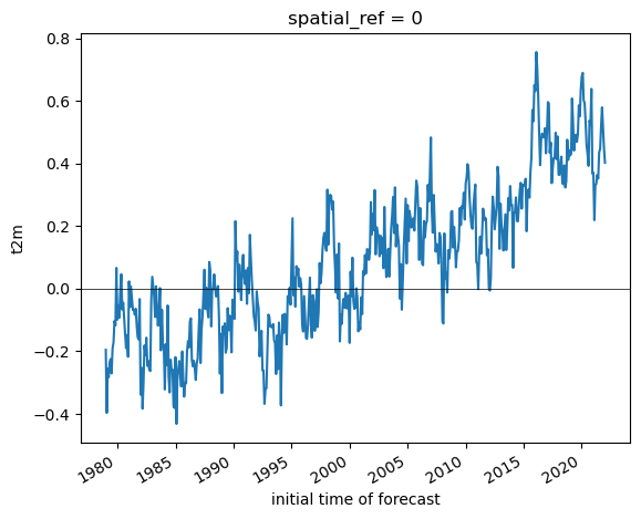
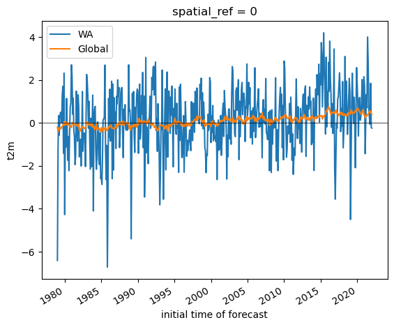
Create a line plot of mean global monthly temperature anomaly from 1979-present#
This should be a simple one-liner
Note: if you used xarray’s default lazy load of the
ncfile, and this is the first time reading the entiret_anom_dsfrom disk, this may take ~20 seconds
#Compute the mean anomaly time series
#Doing this in separate cell, as computing on the fly while plotting consumes a lot of memory
t_anom_da_global = t_anom_da.mean(dim=(xdim, ydim)).compute()
#Student Exercise
#Student Exercise
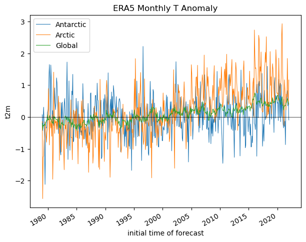
Did the Arctic and Antarctic warm at the same rate over the past 40 years?#
Create a line plot showing anomalies for each region, you can reuse indices from above
t_anom_da_antarctic = t_anom_da.where(antarctic_idx, drop=True).mean(dim=(xdim, ydim)).compute()
t_anom_da_arctic = t_anom_da.where(arctic_idx, drop=True).mean(dim=(xdim, ydim)).compute()
#t_anom_da_nonpolar = t_anom_da.where(nonpolar_idx, drop=True).mean(dim=(xdim, ydim))
f, ax = plt.subplots(figsize=(7,5))
kwargs = {'lw':0.75,'ls':'-'}
t_anom_da_antarctic.plot(ax=ax, label='Antarctic', **kwargs)
t_anom_da_arctic.plot(ax=ax, label='Arctic', **kwargs)
#t_anom_da_nonpolar.plot(ax=ax, label='Non-polar', **kwargs)
t_anom_da_global.plot(ax=ax, label='Global', **kwargs)
ax.axhline(0, color='k', lw=0.5)
ax.set_title('ERA5 Monthly T Anomaly')
ax.legend();
#ax.set_xlim('2015-01-01','2019-01-01')
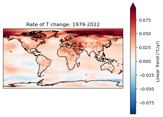
Extra credit: compute linear temperature trend at each pixel and create a map with coastlines#
Note: can coarsen the data to 1x1° to improve performance (16x!)
See the xarray
polyfitfunction: https://docs.xarray.dev/en/stable/generated/xarray.DataArray.polyfit.htmlA linear fit is degree 1
This will return two coefficients (m and b in y=mx+b), so we want to consider m here
t_anom_ds.dims
Frozen({'time': 517, 'latitude': 721, 'longitude': 1440})
ds_factor=4
t_anom_ds_1deg = t_anom_ds.coarsen(latitude=ds_factor, longitude=ds_factor, boundary='trim').mean()
t_anom_ds_1deg.dims
Frozen({'time': 517, 'latitude': 180, 'longitude': 360})
#The difference along the time axis will return values in degrees C per timedelta64[ns] - nanoseconds
#We want degrees C per year
#Conversion factor from nanoseconds to year
dt_factor = 1E9 * (60*60*24*365.25)
#Student Exercise
#Student Exercise
years = pd.DatetimeIndex(t_anom_ds_1deg.time.values).year
#Student Exercise
Text(0.5, 1.0, 'Rate of T change: 1979-2022')
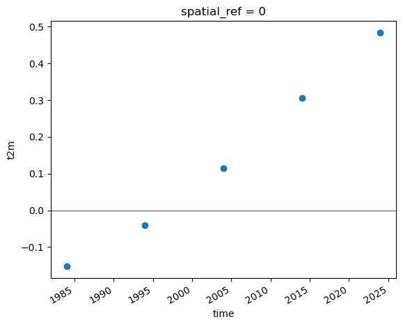
Extra credit: Group temperature anomalies by decade#
See pandas/xarray
resamplefunctionRelevant aliases: https://pandas.pydata.org/pandas-docs/stable/user_guide/timeseries.html#dateoffset-objects
How does the most recent decade compare with the first decade in the time series?
Note that first or last decade in the record might not be “complete” with 10 full years
#Student Exercise
#Student Exercise
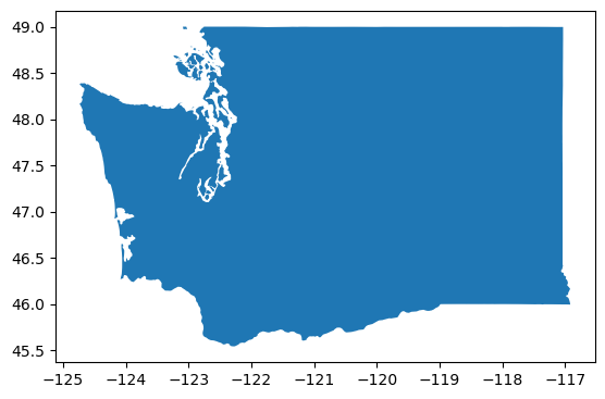
Clip to WA state#
Get the WA state outline#
#states_url = 'http://eric.clst.org/assets/wiki/uploads/Stuff/gz_2010_us_040_00_5m.json'
states_url = 'http://eric.clst.org/assets/wiki/uploads/Stuff/gz_2010_us_040_00_500k.json'
states_gdf = gpd.read_file(states_url)
wa_state = states_gdf.loc[states_gdf['NAME'] == 'Washington']
wa_state.plot();
wa_geom = wa_state.iloc[0].geometry
wa_geom

Get rounded bounds on same grid as ERA5#
wa_bounds = wa_state.total_bounds
wa_bounds
array([-124.733174, 45.543541, -116.915989, 49.002494])
def myround(x, base=0.25):
    return base * np.round(x/base)

def roundbounds(bounds, base=0.25):
    bounds_floor = np.floor(bounds/base)*base
    bounds_ceil = np.ceil(bounds/base)*base
    return [bounds_floor[0], bounds_floor[1], bounds_ceil[2], bounds_ceil[3]]
wa_rbounds = roundbounds(wa_bounds)
wa_rbounds
[-124.75, 45.5, -116.75, 49.25]
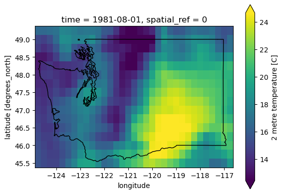
Clip with bounding box selection#
t_clim_ds_wa = t_clim_ds.sel(latitude=slice(wa_rbounds[3],wa_rbounds[1]), longitude=slice(wa_rbounds[0],wa_rbounds[2]))
t_anom_ds_wa = t_anom_ds.sel(latitude=slice(wa_rbounds[3],wa_rbounds[1]), longitude=slice(wa_rbounds[0],wa_rbounds[2]))
f, ax = plt.subplots()
t_clim_ds_wa['t2m'].sel(time=ts).plot(ax=ax, robust=True);
wa_state.plot(ax=ax, edgecolor='k', facecolor='none');
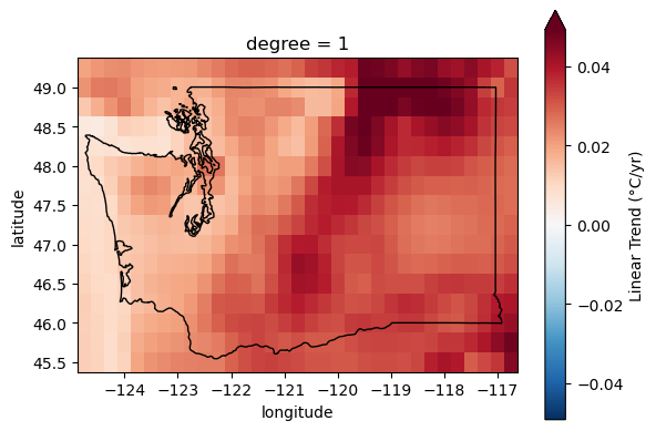
Extra credit: Compute linear temperature trend for WA state#
How does this compare with the global temperature trends?
#Student Exercise
fit = t_anom_ds_wa['t2m'].polyfit(dim='time', deg=1)['polyfit_coefficients']
fit['degree'==1] *= dt_factor
fit.name = 'Linear Trend (°C/yr)'
f, ax = plt.subplots()
fit.sel(degree=1).plot(ax=ax, robust=True, cmap='RdBu_r', center=0);
wa_state.plot(ax=ax, edgecolor='k', facecolor='none');