Demo: Raster fundamentals, Rasterio, Band Math with Arrays
Contents
Demo: Raster fundamentals, Rasterio, Band Math with Arrays#
UW Geospatial Data Analysis
CEE467/CEWA567
David Shean
Introduction#
See reading assignment 05_Raster1_GDAL_rasterio_LS8_prep
What is a raster?#
Raster data sources#
Satellite imagery
Gridded model output
Interpolated vector data
Raster fundamentals#
Interactive discussion during demo
Dimensions (width [columns] and height [rows] in pixels)#
CRS (coordinate system)#
Extent (bounds)#
Resolution (pixel size)#
Data type (bit depth)#
Number of bands#
NoData values#
GDAL (Geospatial Data Abstraction Library) and Rasterio#
GDAL is a powerful and mature library for reading, writing and warping raster datasets, written in C++ with bindings to other languages. There are a variety of geospatial libraries available on the python package index, and almost all of them depend on GDAL. One such python library developed and supported by Mapbox, rasterio, builds on top of GDAL’s many features, but provides a more pythonic interface and supports many of the features and formats that GDAL supports. Both GDAL and rasterio are constantly being updated and improved.
Raster formats#
GeoTiff is most common
GDAL is the foundation - drivers for hundreds of formats
CRS and Projections#
Most often UTM
PROJ is the foundation (as with GeoPandas)
Raster transformations#
Sensor to orthorectified raster image#
Consider the simple example of a 2D detector in a simple camera (e.g., Planet Dove)
Takes a “snapshot” of the Earth surface
A “camera model” or “sensor model” allows you to relate each pixel in the 2D image acquired by the detector to corresponding geographic locations on the ground
Can then create an orthorectified image in some projected coordinate system (like Google Satellite basemap) using a DEM - corrects for perspective, terrain variations
The orthoimage is still a 2D image on the disk, with different number of rows and columns than the original 2D image in sensor coordinates
now “georeferenced” with metadata for the map coordiantes of the upper left pixel and the ground sample distance of each pixel
Orthorectified raster image to projected map coordinates (where we start with Landsat L2 products)#
Need a way to go from pixel coordinates (2D rectangular image on your screen) to real-world coordinates (projected)
Image pixel coordinate system: image width, height in units of pixels, origin (0,0) in upper left corner
Projected coordinate system: “real-world” coordinate system (e.g., UTM 10N) with units of meters and origin (0,0) defined by the CRS (e.g., equator and prime meridian)
Origin is usually upper left corner of upper left pixel
Careful about this - you will definitely run into this problem at some point
Some raster datasets may be shifted by a half a pixel in x and y - upper left corner of upper left pixel vs. center of upper left pixel
Negative y cell size - what’s up with that?
Historical system used by early displays: https://en.wikipedia.org/wiki/Raster_scan
rasterio affine#
Multiply affine by raster (row, col) values to get projected coordinates
Rasterio dataset
xyandindexmethods
GDAL/ESRI affine#
Basic raster structure#
Dataset object
Open to access metadata, doesn’t read pixels
Bands
Often just 1 band, sometimes multiple bands in a single Dataset (new axis)
Can read individual bands to access corresponding 2D array data
Handling missing data (nodata) - masked arrays vs. np.nan
Overviews#
3D array to create composites from multispectral bands#
Can dstack 2D arrays
Will revisit with
rioxarray
Misc#
Be careful with large rasters, esp float - don’t load into memory
Read in a window or every nth pixel when prototyping. Only read in full res when code is working for smaller raster.
Try to avoid creating many copies of arrays, close datasets no longer needed
GDAL command line utilities#
Most common tools to learn:
gdalinfo
gdal_translate
gdalwarp
gdaladdo
Items to discuss
Use standard creation options (co)
TILED=YES
COMPRESS=LZW
BIGTIFF=IF_SAFER
Resampling algorithms
Default is nearest
Often bilinear or bicubic is a better choice for reprojecting, upsampling, downsampling
Demo#
https://automating-gis-processes.github.io/site/notebooks/Raster/reading-raster.html
pwd
'/home/jovyan/jupyterbook/book/modules/05_Raster1_GDAL_rasterio_LS8'
import os
import numpy as np
import matplotlib.pyplot as plt

import rasterio as rio
import rasterio.plot
from osgeo import gdal

#Useful package to add dynamic scalebar to matplotlib images
from matplotlib_scalebar.scalebar import ScaleBar
#We want to use interactive plotting for zoom/pan and live coordinate display
#%matplotlib widget
%matplotlib inline
#Create local directory to store images
imgdir = 'LS8_sample'

#Pre-identified cloud-free Image IDs used for the lab
#Summer 2018
img_id1 = 'LC08_L2SP_046027_20180818_20200831_02_T1'
#Winter 2018
img_id2 = 'LC08_L2SP_046027_20181224_20200829_02_T1'

img = img_id1
Let’s use the Thermal IR band for this demo#
#Specify filenames for different bands we will need for the lab
#Check table from background section to see wavelengths of each band number
tir_fn = os.path.join(imgdir, img+'_ST_B10.TIF')
print(tir_fn)
LS8_sample/LC08_L2SP_046027_20180818_20200831_02_T1_ST_B10.TIF
!gdalinfo $tir_fn
Driver: GTiff/GeoTIFF
Files: LS8_sample/LC08_L2SP_046027_20180818_20200831_02_T1_ST_B10.TIF
Size is 7771, 7891
Coordinate System is:
PROJCRS["WGS 84 / UTM zone 10N",
    BASEGEOGCRS["WGS 84",
        DATUM["World Geodetic System 1984",
            ELLIPSOID["WGS 84",6378137,298.257223563,
                LENGTHUNIT["metre",1]]],
        PRIMEM["Greenwich",0,
            ANGLEUNIT["degree",0.0174532925199433]],
        ID["EPSG",4326]],
    CONVERSION["UTM zone 10N",
        METHOD["Transverse Mercator",
            ID["EPSG",9807]],
        PARAMETER["Latitude of natural origin",0,
            ANGLEUNIT["degree",0.0174532925199433],
            ID["EPSG",8801]],
        PARAMETER["Longitude of natural origin",-123,
            ANGLEUNIT["degree",0.0174532925199433],
            ID["EPSG",8802]],
        PARAMETER["Scale factor at natural origin",0.9996,
            SCALEUNIT["unity",1],
            ID["EPSG",8805]],
        PARAMETER["False easting",500000,
            LENGTHUNIT["metre",1],
            ID["EPSG",8806]],
        PARAMETER["False northing",0,
            LENGTHUNIT["metre",1],
            ID["EPSG",8807]]],
    CS[Cartesian,2],
        AXIS["(E)",east,
            ORDER[1],
            LENGTHUNIT["metre",1]],
        AXIS["(N)",north,
            ORDER[2],
            LENGTHUNIT["metre",1]],
    USAGE[
        SCOPE["Engineering survey, topographic mapping."],
        AREA["Between 126°W and 120°W, northern hemisphere between equator and 84°N, onshore and offshore. Canada - British Columbia (BC); Northwest Territories (NWT); Nunavut; Yukon. United States (USA) - Alaska (AK)."],
        BBOX[0,-126,84,-120]],
    ID["EPSG",32610]]
Data axis to CRS axis mapping: 1,2
Origin = (473685.000000000000000,5373615.000000000000000)
Pixel Size = (30.000000000000000,-30.000000000000000)
Metadata:
  AREA_OR_POINT=Point
Image Structure Metadata:
  COMPRESSION=DEFLATE
  INTERLEAVE=BAND
Corner Coordinates:
Upper Left  (  473685.000, 5373615.000) (123d21'22.79"W, 48d30'54.35"N)
Lower Left  (  473685.000, 5136885.000) (123d20'32.02"W, 46d23' 6.10"N)
Upper Right (  706815.000, 5373615.000) (120d12' 4.44"W, 48d28'53.80"N)
Lower Right (  706815.000, 5136885.000) (120d18'42.66"W, 46d21'14.16"N)
Center      (  590250.000, 5255250.000) (121d48'10.55"W, 47d26'40.00"N)
Band 1 Block=256x256 Type=UInt16, ColorInterp=Gray
  NoData Value=0
  Overviews: 3886x3946, 1943x1973, 972x987, 486x494, 243x247, 122x124
  Offset: 149,   Scale:0.00341802
Rasterio basics#
We’ll stick with rasterio for most of our Python raster analysis
Use a Python with construct to cleanly open, inspect, and close the file directly from the url#
The Python
withconstruct may be new, or maybe you used it during Lab02 when opening a text file for reading/writing.It is “used in exception handling to make the code cleaner and much more readable. It simplifies the management of common resources like file streams.”
Enables more elegant file opening/closing and handling errors (like missing files)
Let’s use the
with rio.open()approach to print out the rasterio dataset profile, without actually reading the underlying image dataWe will temporarily store the rasterio dataset with variable name
src(short for “source”)
with rio.open(tir_fn) as src:
    print(src.profile)
{'driver': 'GTiff', 'dtype': 'uint16', 'nodata': 0.0, 'width': 7771, 'height': 7891, 'count': 1, 'crs': CRS.from_epsg(32610), 'transform': Affine(30.0, 0.0, 473685.0,
       0.0, -30.0, 5373615.0), 'blockxsize': 256, 'blockysize': 256, 'tiled': True, 'compress': 'deflate', 'interleave': 'band'}
Can also open dataset with rasterio for persistence and interactive access#
This is likely a better option as you’re learning, as you can access the opened dataset and arrays you’ve already read in other cells
Remember to close the rasterio dataset when no longer needed!
src = rio.open(tir_fn)
type(src)
rasterio.io.DatasetReader
src.profile
{'driver': 'GTiff', 'dtype': 'uint16', 'nodata': 0.0, 'width': 7771, 'height': 7891, 'count': 1, 'crs': CRS.from_epsg(32610), 'transform': Affine(30.0, 0.0, 473685.0,
       0.0, -30.0, 5373615.0), 'blockxsize': 256, 'blockysize': 256, 'tiled': True, 'compress': 'deflate', 'interleave': 'band'}
src.meta
{'driver': 'GTiff',
 'dtype': 'uint16',
 'nodata': 0.0,
 'width': 7771,
 'height': 7891,
 'count': 1,
 'crs': CRS.from_epsg(32610),
 'transform': Affine(30.0, 0.0, 473685.0,
        0.0, -30.0, 5373615.0)}
src.crs
CRS.from_epsg(32610)
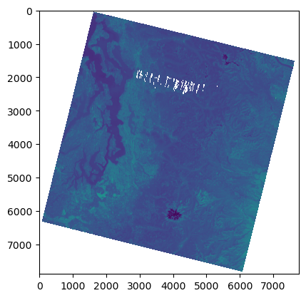
Plot using rasterio show() function#
Note axes tick labels
rio.plot.show(src);

Read the array#
#src.read?
#Note memory usage before and after reading
%time
a = src.read(1)
CPU times: user 2 µs, sys: 1 µs, total: 3 µs
Wall time: 7.63 µs
a
array([[0, 0, 0, ..., 0, 0, 0],
       [0, 0, 0, ..., 0, 0, 0],
       [0, 0, 0, ..., 0, 0, 0],
       ...,
       [0, 0, 0, ..., 0, 0, 0],
       [0, 0, 0, ..., 0, 0, 0],
       [0, 0, 0, ..., 0, 0, 0]], dtype=uint16)
a.shape
(7891, 7771)
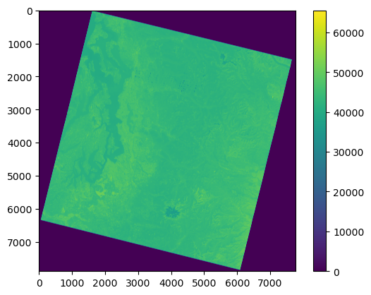
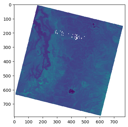
Plot using Matplotlib imshow#
Note axes tick labels
f,ax = plt.subplots()
m = ax.imshow(a)
plt.colorbar(m, ax=ax);
Inspect the array#
a.shape
(7891, 7771)
a.size
61320961
a.dtype
dtype('uint16')
a.min()
0
a.max()
65535
2**16
65536
a.shape
(7891, 7771)
#Convert to 1D (needed for histogram)
a.ravel().shape
(61320961,)
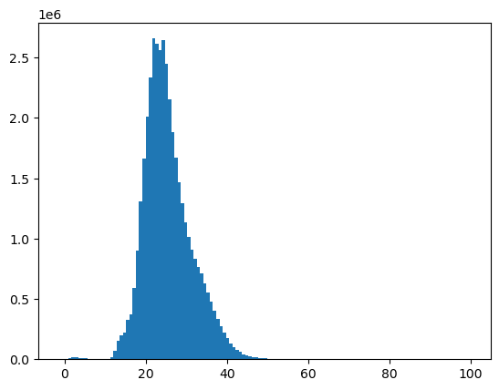
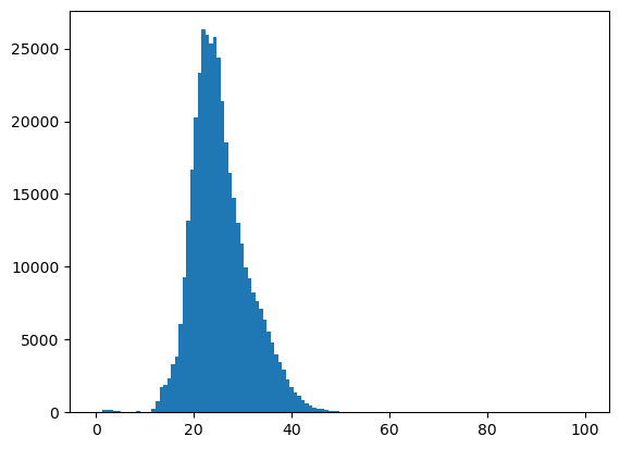
f, ax = plt.subplots()
ax.hist(a.ravel(), bins=128);
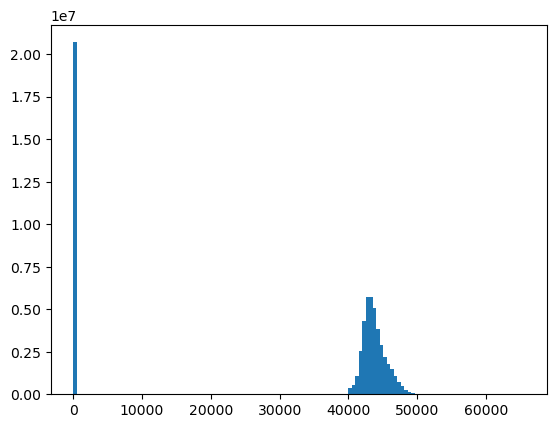
Data type and bit depth#
Note values in histogram - 16 bit integer vs. 12 bit dynamic range of instrument
2**16
65536
#Landsat-8 OLI is 12-bit sensor
2**12
4096
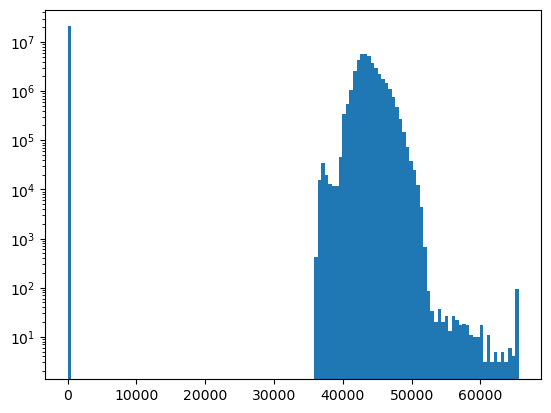
f, ax = plt.subplots()
ax.hist(a.ravel(), bins=128, log=True);
Use a masked array to handle nodata#
src.profile
{'driver': 'GTiff', 'dtype': 'uint16', 'nodata': 0.0, 'width': 7771, 'height': 7891, 'count': 1, 'crs': CRS.from_epsg(32610), 'transform': Affine(30.0, 0.0, 473685.0,
       0.0, -30.0, 5373615.0), 'blockxsize': 256, 'blockysize': 256, 'tiled': True, 'compress': 'deflate', 'interleave': 'band'}
src.nodata
0.0
src.nodatavals
(0.0,)
#If nodata is defined, rasterio can created masked array when reading
src.read(1, masked=True)
masked_array(
  data=[[--, --, --, ..., --, --, --],
        [--, --, --, ..., --, --, --],
        [--, --, --, ..., --, --, --],
        ...,
        [--, --, --, ..., --, --, --],
        [--, --, --, ..., --, --, --],
        [--, --, --, ..., --, --, --]],
  mask=[[ True,  True,  True, ...,  True,  True,  True],
        [ True,  True,  True, ...,  True,  True,  True],
        [ True,  True,  True, ...,  True,  True,  True],
        ...,
        [ True,  True,  True, ...,  True,  True,  True],
        [ True,  True,  True, ...,  True,  True,  True],
        [ True,  True,  True, ...,  True,  True,  True]],
  fill_value=0,
  dtype=uint16)
#Can also create from existing NumPy array
#np.ma.masked_equal?
np.ma.masked_equal(a, 0)
masked_array(
  data=[[--, --, --, ..., --, --, --],
        [--, --, --, ..., --, --, --],
        [--, --, --, ..., --, --, --],
        ...,
        [--, --, --, ..., --, --, --],
        [--, --, --, ..., --, --, --],
        [--, --, --, ..., --, --, --]],
  mask=[[ True,  True,  True, ...,  True,  True,  True],
        [ True,  True,  True, ...,  True,  True,  True],
        [ True,  True,  True, ...,  True,  True,  True],
        ...,
        [ True,  True,  True, ...,  True,  True,  True],
        [ True,  True,  True, ...,  True,  True,  True],
        [ True,  True,  True, ...,  True,  True,  True]],
  fill_value=0,
  dtype=uint16)
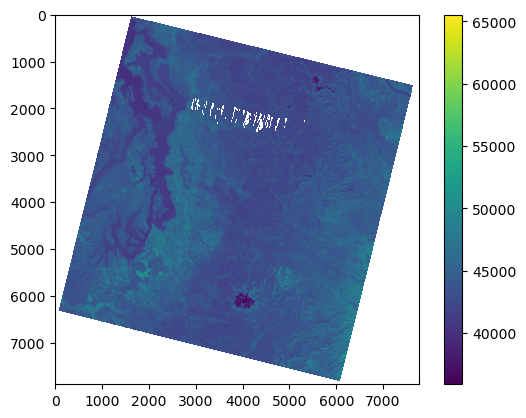
a = np.ma.masked_equal(a, 0)
f,ax = plt.subplots()
m = ax.imshow(a)
plt.colorbar(m, ax=ax);
f, ax = plt.subplots()
ax.hist(a.compressed(), bins=128);

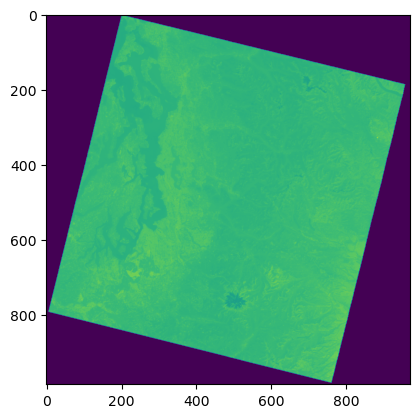
Scaling 16-bit values to geophysical variables - surface reflectance and temperature#
Use raster math to multiply by scaling factor and add offset value
See conversion factors here: https://www.usgs.gov/landsat-missions/landsat-collection-2-level-2-science-products
https://www.usgs.gov/faqs/how-do-i-use-scale-factor-landsat-level-2-science-products
Units:
Unitless surface reflectance values from 0.0 to 1.0
Surface temperature values in Kelvin - can convert to Celsius
#Notes on attemting to apply scale and offset dynamically
#mode='r+', scales=(st_scale,), offsets=(st_offset,), mask_and_scale=True
#src.scales = (st_scale,)
#src.offsets = (st_offset,)
#src.scales, src.offsets
#These are the standard scale and offset values
#SR 0.0000275 + -0.2
sr_scale = 0.0000275
sr_offset = -0.2
#ST 0.00341802 + 149.0
st_scale = 0.00341802
st_offset = 149.0
#We are working with Thermal IR band, so let's use the thermal scale and offset
a_st = a * st_scale + st_offset
#Convert to Celsius
a_st -= 273.15
a_st.dtype
dtype('float64')
a_st.min()
-1.4294099200000119
#Float16 should provide enough precision for these data
a_st = a_st.astype('float32')
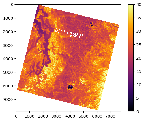
f, ax = plt.subplots()
plt.hist(a_st.compressed(), bins=128);
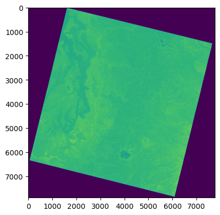
#%matplotlib widget
f, ax = plt.subplots()
m = ax.imshow(a_st, vmin=0, vmax=40, cmap='inferno')
plt.colorbar(m, ax=ax);
Bounds and extent#
#This is rasterio bounds object in projected units (meters) - note labels like dictionary keys and values
src.bounds
BoundingBox(left=473685.0, bottom=5136885.0, right=706815.0, top=5373615.0)
#This is matplotlib extent
full_extent = [src.bounds.left, src.bounds.right, src.bounds.bottom, src.bounds.top]
print(full_extent)
[473685.0, 706815.0, 5136885.0, 5373615.0]
#rasterio convenience function
full_extent = rio.plot.plotting_extent(src)
print(full_extent)
(473685.0, 706815.0, 5136885.0, 5373615.0)
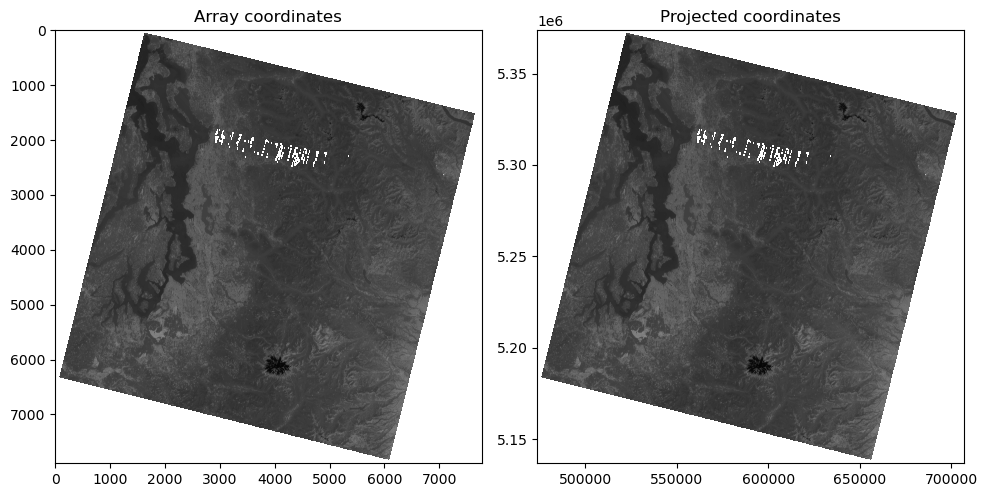
Plot the image with matplotlib imshow, but now pass in this extent as an argument#
Note how the axes coordinates change
These should now be meters in the UTM 10N coordinate system of the projected image!
f, axa = plt.subplots(1,2, figsize=(10,6))
axa[0].imshow(a, cmap='gray') #vmin=0, vmax=1
axa[0].set_title("Array coordinates")
axa[1].imshow(a, extent=full_extent, cmap='gray') #vmin=0, vmax=1
axa[1].set_title("Projected coordinates")
plt.tight_layout()
Raster transform#
How does rasterio know the bounds?
Inspect the dataset
transformattributeYou may have encountered an ESRI “world file” or GDAL geotransform before. This is the same idea, but Rasterio’s model uses traditional affine transform.
Review this: https://rasterio.readthedocs.io/en/stable/topics/georeferencing.html?highlight=affine#coordinate-transformation
src.transform
Affine(30.0, 0.0, 473685.0,
       0.0, -30.0, 5373615.0)
#These are (x,y) for corners in image/array coordinates (pixels)
#A bit confusing due to (row,col) of shape, which is (y,x)

#Upper left
ul = (0, 0)
#One pixel from upper left
ul1 = (1,1)
#Lower right
lr = (a_st.shape[1], a_st.shape[0])

print(ul, ul1, lr)
(0, 0) (1, 1) (7771, 7891)
#Transform upper left corner to projected coordinates (meters)
print(ul)
ul_proj = src.transform * ul
print(ul_proj)
(0, 0)
(473685.0, 5373615.0)
#Transform the one pixel offset from ul to projected coordinates (meters)
print(ul1)
ul1_proj = src.transform * ul1
print(ul1_proj)
(1, 1)
(473715.0, 5373585.0)
np.array(ul_proj) - np.array(ul1_proj)
array([-30., 30.])
#Transform lower right corner
print(lr)
lr_proj = src.transform * lr
print(lr_proj)
(7771, 7891)
(706815.0, 5136885.0)
wh_km = np.abs(np.array(ul_proj) - np.array(lr_proj))/1000
wh_km
print('Total width: %0.2f km\nTotal height: %0.2f km' % (wh_km[0], wh_km[1]))
Total width: 233.13 km
Total height: 236.73 km
Raster and array sampling#
Use helper functions
xyandsample
a_st
masked_array(
  data=[[--, --, --, ..., --, --, --],
        [--, --, --, ..., --, --, --],
        [--, --, --, ..., --, --, --],
        ...,
        [--, --, --, ..., --, --, --],
        [--, --, --, ..., --, --, --],
        [--, --, --, ..., --, --, --]],
  mask=[[ True,  True,  True, ...,  True,  True,  True],
        [ True,  True,  True, ...,  True,  True,  True],
        [ True,  True,  True, ...,  True,  True,  True],
        ...,
        [ True,  True,  True, ...,  True,  True,  True],
        [ True,  True,  True, ...,  True,  True,  True],
        [ True,  True,  True, ...,  True,  True,  True]],
  fill_value=0.0,
  dtype=float32)
a_st[0,0]
masked
#Array coordinates
c = (3512, 3512)
#Get value at coordinates using array indexing
a_st[c[0], c[1]]
23.241858
#src.xy?
#Note use of argument expansion here (*c) so we don't have to pass individual c[0] and c[1] values
x,y = src.xy(*c)
print(x,y)
579060.0 5268240.0
#a_st[int(x), int(y)]
#src.sample?
#Doesn't actually produce coordinates
src.sample(x, y)
<generator object sample_gen at 0x7f1da44a0580>
#Doesn't work - need to pass in list
#list(src.sample(x, y))
src.sample([(x, y),])
<generator object sample_gen at 0x7f1da44a05f0>
#Pass in a list of (x,y) coordinate pairs, and evaluate the generator
list(src.sample([(x, y),]))
[array([43122], dtype=uint16)]
s = list(src.sample([(x, y), (x+30, y+30), (x-30, y-30)]))
s
[array([43122], dtype=uint16),
 array([43144], dtype=uint16),
 array([43093], dtype=uint16)]
s[0]
array([43122], dtype=uint16)
np.array(s).squeeze()
array([43122, 43144, 43093], dtype=uint16)
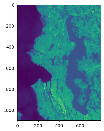
Windowing and indexing#
chunk = a_st[2700:3800,2200:3000]
chunk
masked_array(
  data=[[15.855517387390137, 15.930713653564453, 16.036672592163086, ...,
         33.80695724487305, 33.171207427978516, 33.08575439453125],
        [15.927295684814453, 15.98198413848877, 16.050344467163086, ...,
         33.60187530517578, 32.596981048583984, 32.29277420043945],
        [15.99565601348877, 16.029836654663086, 16.077688217163086, ...,
         33.41730499267578, 32.17656326293945, 31.63651466369629],
        ...,
        [22.681303024291992, 22.616361618041992, 22.60610580444336, ...,
         30.946075439453125, 28.891845703125, 27.948471069335938],
        [22.900056838989258, 22.715482711791992, 22.691556930541992, ...,
         30.67947006225586, 29.110599517822266, 28.5192813873291],
        [22.947908401489258, 22.718900680541992, 22.732572555541992, ...,
         30.580347061157227, 30.026628494262695, 29.83521842956543]],
  mask=[[False, False, False, ..., False, False, False],
        [False, False, False, ..., False, False, False],
        [False, False, False, ..., False, False, False],
        ...,
        [False, False, False, ..., False, False, False],
        [False, False, False, ..., False, False, False],
        [False, False, False, ..., False, False, False]],
  fill_value=0.0,
  dtype=float32)
f, ax = plt.subplots()
plt.imshow(chunk, interpolation='none')
<matplotlib.image.AxesImage at 0x7f1da431c310>
Store a reduced resolution view (1 pixel for every 100 original pixels)#
asub = a_st[::10, ::10]
asub
masked_array(
  data=[[--, --, --, ..., --, --, --],
        [--, --, --, ..., --, --, --],
        [--, --, --, ..., --, --, --],
        ...,
        [--, --, --, ..., --, --, --],
        [--, --, --, ..., --, --, --],
        [--, --, --, ..., --, --, --]],
  mask=[[ True,  True,  True, ...,  True,  True,  True],
        [ True,  True,  True, ...,  True,  True,  True],
        [ True,  True,  True, ...,  True,  True,  True],
        ...,
        [ True,  True,  True, ...,  True,  True,  True],
        [ True,  True,  True, ...,  True,  True,  True],
        [ True,  True,  True, ...,  True,  True,  True]],
  fill_value=0.0,
  dtype=float32)
asub.shape
(790, 778)
%time
f, ax = plt.subplots()
plt.imshow(a_st);
CPU times: user 3 µs, sys: 0 ns, total: 3 µs
Wall time: 7.87 µs
#Every 10th pixel - great strategy for quick visualization during development/exploration
%time
f, ax = plt.subplots()
plt.imshow(asub);
CPU times: user 3 µs, sys: 0 ns, total: 3 µs
Wall time: 7.39 µs
Reading in reduced resolution overview from the start#
Since we have a cloud optimized geotiff (COG), can directly read the embedded overviews, rather than full resolution data
Easier with rioxarray (later)
ovr_level = 8 #power of 2 (see gdalinfo above for overview dimensions)
ovr_shape = (int(src.height/ovr_level), int(src.width/ovr_level))
#Note memory usage before and after reading
%time
a_ovr = src.read(1, out_shape=ovr_shape)
CPU times: user 4 µs, sys: 0 ns, total: 4 µs
Wall time: 7.39 µs
t = src.transform
t
Affine(30.0, 0.0, 473685.0,
       0.0, -30.0, 5373615.0)
#Should assign this to new dataset/profile for ovr (or just use rioxarray)
import affine
ovr_transform = affine.Affine(t[0]*ovr_level, t[1], t[2], t[3], t[4]*ovr_level, t[5])
ovr_transform
Affine(240.0, 0.0, 473685.0,
       0.0, -240.0, 5373615.0)
a.shape
(7891, 7771)
a_ovr.shape
(986, 971)
%time
f, ax = plt.subplots()
plt.imshow(a_ovr);
CPU times: user 5 µs, sys: 1e+03 ns, total: 6 µs
Wall time: 12.2 µs
Raster math#
#%matplotlib widget
#Remember to use compressed for historgrams with 2D masked arrays
f, ax = plt.subplots()
plt.hist(asub.compressed(), bins=128);
t_thresh = 18 #Deg C
asub
masked_array(
  data=[[--, --, --, ..., --, --, --],
        [--, --, --, ..., --, --, --],
        [--, --, --, ..., --, --, --],
        ...,
        [--, --, --, ..., --, --, --],
        [--, --, --, ..., --, --, --],
        [--, --, --, ..., --, --, --]],
  mask=[[ True,  True,  True, ...,  True,  True,  True],
        [ True,  True,  True, ...,  True,  True,  True],
        [ True,  True,  True, ...,  True,  True,  True],
        ...,
        [ True,  True,  True, ...,  True,  True,  True],
        [ True,  True,  True, ...,  True,  True,  True],
        [ True,  True,  True, ...,  True,  True,  True]],
  fill_value=0.0,
  dtype=float32)
#Identifiy pixels with values less than some threshold
asub < t_thresh
masked_array(
  data=[[--, --, --, ..., --, --, --],
        [--, --, --, ..., --, --, --],
        [--, --, --, ..., --, --, --],
        ...,
        [--, --, --, ..., --, --, --],
        [--, --, --, ..., --, --, --],
        [--, --, --, ..., --, --, --]],
  mask=[[ True,  True,  True, ...,  True,  True,  True],
        [ True,  True,  True, ...,  True,  True,  True],
        [ True,  True,  True, ...,  True,  True,  True],
        ...,
        [ True,  True,  True, ...,  True,  True,  True],
        [ True,  True,  True, ...,  True,  True,  True],
        [ True,  True,  True, ...,  True,  True,  True]],
  fill_value=0.0)
f, ax = plt.subplots()
plt.imshow(asub <= t_thresh);
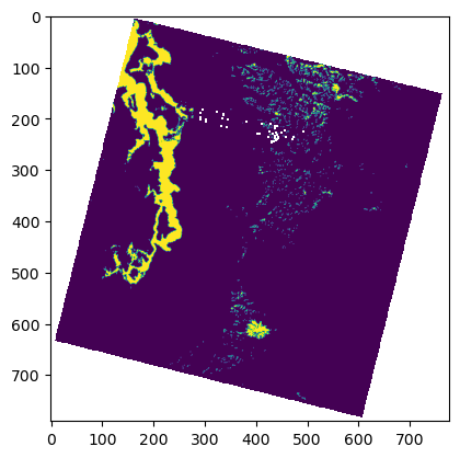
#Use nearest neighbor interpolation for binary raster data!
plt.imshow(asub <= t_thresh, interpolation='none');

Calculating area#
a_st.size
61320961
a_st.compressed().size
40633950
a_st.count()
40633950
#Count up nonzero values - somewhat complicated way
(a_st <= t_thresh).nonzero()[0].size
2512952
#Sum the boolean values (True = 1, False = 0)
n_px = (a_st <= t_thresh).sum()
n_px
2512952
src.res
(30.0, 30.0)
#Ground sample distance for a single pixel in meters
src.res
(30.0, 30.0)
#Area of single pixel (m^2)
px_area = src.res[0] * src.res[1]
px_area
900.0
n_px * px_area
2261656800.0
Cleanup and memory management#
#Delete array from memory
a = None
a_st = None
asub = None
#Close the rasterio dataset
src.close()
#%reset array
GDAL Python API basics#
I’m including this for reference
It’s not that complicated, even though rasterio is the more popular option for Python these days (partly because of much better documentation)
https://github.com/OSGeo/gdal/tree/master/gdal/swig/python/samples
#Open the green band GeoTiff as GDAL Dataset object
ds = gdal.Open(tir_fn)
#Get the raster band
gdal_b = ds.GetRasterBand(1)
#Read into array
a = gdal_b.ReadAsArray()
#Inspect the array
a
array([[0, 0, 0, ..., 0, 0, 0],
       [0, 0, 0, ..., 0, 0, 0],
       [0, 0, 0, ..., 0, 0, 0],
       ...,
       [0, 0, 0, ..., 0, 0, 0],
       [0, 0, 0, ..., 0, 0, 0],
       [0, 0, 0, ..., 0, 0, 0]], dtype=uint16)
#View the array
f, ax = plt.subplots()
ax.imshow(a);
#Set array to None (frees up RAM) and close GDAL dataset
a = None
ds = None