Lab05 Exercises #1
Contents
Lab05 Exercises #1#
UW Geospatial Data Analysis
CEE467/CEWA567
David Shean
Objectives#
Learn how to inspect, read and write raster data
Develop a more intuitive understanding of raster transforms, window/extent operations
Understand raster visualization approaches, contrast stretching and interpolation settings
Perform common raster band math operations (e.g., NDVI) using NumPy
Perform quantitative raster analysis using value thresholds and binary masks
Understand programmtic Landsat-8 archive access and download
import os
import numpy as np
import matplotlib.pyplot as plt

import rasterio as rio
import rasterio.plot
from osgeo import gdal

#Useful package to add dynamic scalebar to matplotlib images
from matplotlib_scalebar.scalebar import ScaleBar
Part 0: Run Landsat data download notebook, set path to data directory#
05_Raster1_LS8_download.ipynb
pwd
'/home/jovyan/src/gda_course_2023_solutions/modules/05_Raster1_GDAL_rasterio_LS8'
#Open accompanying notebook and Run All Cells
#Alternatively, can run from this notebook, which should preserve variables/state
#%run ./05_Raster1_LS8_download.ipynb
#Set path to local directory with downloaded images
imgdir = '/home/jovyan/jupyterbook/book/modules/05_Raster1_GDAL_rasterio_LS8/LS8_sample'
#Pre-identified cloud-free Image IDs used for the lab
#Summer 2018
img_id1 = 'LC08_L2SP_046027_20180818_20200831_02_T1'
#Winter 2018
img_id2 = 'LC08_L2SP_046027_20181224_20200829_02_T1'
#Define image to use (can set this to switch to winter image)
img = img_id1
#Red band filename
r_fn = os.path.join(imgdir, img+'_SR_B4.TIF')
Part 1: Raster basics#
Open the downloaded image from disk#
Since we already downloaded these images locally, let’s just open a local file
Let’s use of the red band (B4) TIF file
We already defined the
r_fnabove, so this should be easy
Don’t use the
withconstruct - store the opened dataset in a variable, so we can use in other cells
print(r_fn)
src = rio.open(r_fn)
What is the CRS of the dataset?#
Look familiar? The
fionafunctionality underlyingrasterio(also used bygeopandas) was mostly written by the same author (Sean Gilles, https://github.com/sgillies).If you don’t recognize it by now, take a minute to look up this EPSG code
#Student Exercise
What is the raster extent (bounds) of the dataset in projected coordinates?#
Note that this is not a simple python
listobject, but a special rasterioBoundingBoxobject with attributes forleft,bottom, etc.This helps you avoid mixing up order of values that correspond to
(min_x, min_y, max_x, max_y)Note that other API and utilities may use different order (e.g.,
min_x, max_x, min_y, max_y)
#Student Exercise
#Student Exercise
How many bands are there in this dataset?#
Check the approprate rasterio dataset attribute
#Student Exercise
Review the profile and metadata record#
Inspect the rasterio
profileandmetaattributes, which should return dictionaries for all metadata
#Student Exercise
#Student Exercise
OK, let’s read the raster data into a NumPy array and preview#
Store the output array as a new variable called
rUse default read options for now, don’t read as masked array
What band number should we use here?
This dataset is for the red Landsat multispectral band, which is band #4 (B4)
But each Landsat band is stored as a separate TIF file (remember your dataset band
countattribute above)So using rasterio
read, which band do you need to load?Note: If you omit the band number, rasterio will return a 3D NumPy array with an additional dimension
#Student Exercise
<class 'numpy.ndarray'>
array([[0, 0, 0, ..., 0, 0, 0],
       [0, 0, 0, ..., 0, 0, 0],
       [0, 0, 0, ..., 0, 0, 0],
       ...,
       [0, 0, 0, ..., 0, 0, 0],
       [0, 0, 0, ..., 0, 0, 0],
       [0, 0, 0, ..., 0, 0, 0]], dtype=uint16)
What are the dimensions of the NumPy array?#
Compare this with the rasterio dataset
widthandheightattributesLook carefully, as these are slightly different
Hopefully this offers a reminder about the ordering of NumPy indices, with (row, col) representing (y,x) dimensions
#Student Exercise
What is the uncompressed filesize of this array in Megabytes?#
You can compute this using the array data type and dimensions
Can check with the NumPy array
nbytesattribute
This is how much RAM the array is occupying after the read operation
How does this compare with the file size of this file on disk (see output from
ls -alh)?If different, why might they be different? ✍️
!ls -lah $r_fn
-rw-rw-r-- 1 jovyan users 83M Feb 1 04:03 /home/jovyan/jupyterbook/book/modules/05_Raster1_GDAL_rasterio_LS8/LS8_sample/LC08_L2SP_046027_20180818_20200831_02_T1_SR_B4.TIF
#Student Exercise
#Student Exercise
Create a plot of the image#
Earlier we used the
rio.plot.show()convenience function for plotting a dataset, which is a wrapper around the standard matplotlibimshow(). Here, let’s create a figure/axes and use matplotlibimshowto view the array.Use the
graycolor ramp (seeimshowdoc on how to specify color ramp)If using
%matplotlib widgetbackend, I recommend you start withf,ax = plt.subplots(), which will create a new figure in the cell (otherwise, yourimshowoutput could end up in an earlier figure).
#%matplotlib widget
#Student Exercise
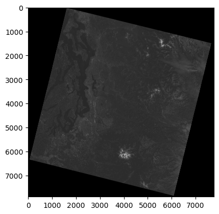
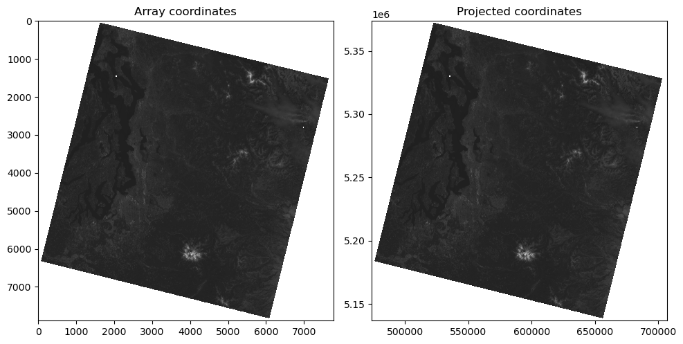
Note that the Landsat-8 image appears “rotated” relative to the axes
Why is this? ✍️
Note the array coordinate system (where is the (0,0) origin)
Interactively look at coordinates and the digital number (DN) values as you move your mouse over the image
The DN is the unsigned integer value, but not yet a calibrated surface reflectance value (which would have dimensionless values over the range 0.0-1.0)
Check DN values over Mt. Rainier, Puget Sound, and the outer “black” border
#Student Exercise
#Student Exercise
Part 2: Histograms, NoData and Masked Arrays#
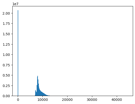
Create a histogram plot of raster values in your array#
Does the matplotlib
hist()expect a 2D array or a 1D array?Remember to use the NumPy
ravel()function on your array when passing tohist()!
Make sure you use enough bins! Try at least ~200.
🤔 Which bin has the highest count of pixels?
🤔 Over what range do most of the raster values fall?
Is this consistent with the original 12-bit sensor bit depth (2^12 possible values) and 16-bit integer data type (2^16 possible values)?
#Student Exercise
src.nodata
0.0
Let’s get rid of that black border (nodata values)#
The Level-2 Landsat-8 images have a
nodatavalue set in the image metadata, but we did not use this when readingAs a result, the 0 values around the margins are considered “valid” pixels, and these appear black in our grayscale color ramp
We have a few options to deal with missing data (read through both before starting):
Set values of 0 to
np.nanRemember that
np.nanis a specialfloatobject, so for this approach, you must first convert the entire array usingastype(float)This means we unnecessarily increase the amount of RAM required to store the same
UInt16(2 byte) image DN values by a factor of 2x or 4x, as eachfloat32value occupies 4 bytes, and the default NumPyfloatis actuallyfloat64or 8 bytes! This increased memory requirement can be a real issue for large arrays.For this reason, I suggest that you work with masked arrays (Option 2) for rasters with integer data types and nodata defined.
Note that there are a growing number of “nan-aware” functions in NumPy (e.g., np.nanpercentile), but still limitations
Note that some packages like Pandas and xarray don’t currently support masked ararys, but rely on
np.nanfor missing values
Use a NumPy masked array (should be simple one-liner)
Take a few minutes to read about masked arrays
https://docs.scipy.org/doc/numpy/reference/maskedarray.generic.html#what-is-a-masked-array
https://docs.scipy.org/doc/numpy/reference/maskedarray.generic.html
Masked arrays allow for masking invalid values on any datatype (like
ByteorUInt16)Stores the mask as an additoinal 1-bit boolean array
See the
masked_equalfunction to create a masked array from an existing array
Use the
masked=Trueoption when reading a band from the rasterio dataset (with NoData properly set)For example
r = src.read(1, masked=True)More info on rasterio nodata handling and more advanced masking support: https://rasterio.readthedocs.io/en/latest/topics/masks.html
Prepare a masked array for the red band using one of the approaches above#
Preview your new array, inspect the mask
Try plotting the masked array with imshow using the
graycmapYou should no longer see a black border around the valid pixels
#Student Exercise
#Student Exercise
#Student Exercise
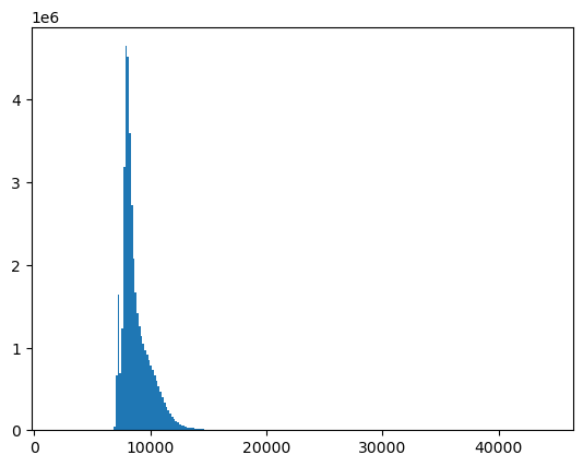
Replot the histogram of your masked array#
Remember to use the new masked array object method
compressed()to pass the unmasked values as a 1D array tohist()There should no longer be a spike for the 0 bin
Experiment with
log=Trueto thehistcall to display logarithmic y axis for the bin counts
#Student Exercise
#Student Exercise
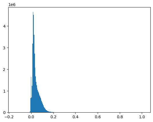
Scale the 16-bit values to geophysical variables - surface reflectance#
We want to multiply the masked array values by the known scaling factor and then add the known offset value - these are provided by the Landsat project
Store the output as a separate array
Unitless surface reflectance values are from 0.0 to 1.0
Sanity check with a histogram
#Surface Reflectance 0.0000275 + -0.2
sr_scale = 0.0000275
sr_offset = -0.2
#Student Exercise
#Student Exercise
Print the min and max values of the original, masked, and scaled arrays#
Note that 0 is no longer the minimum in the scaled values for the masked array
#Student Exercise
Determine 2nd and 98th percentile of surface reflectance values#
These percentile values can be used to automatically set the
vminandvmaxwhen plotting (e.g., in QGIS)Note that if you’re using a masked array, you will need to isolate unmasked values using the
compressed()method before passing to regular NumPy functions likenp.percentilePlot these as vertical dotted black lines on a histogram
Hopefully this helps visualize what these percentile values represent based on your distribution.
#Student Exercise
[-0.002605 0.134785]

Part 3: Raster transform#
Inspect the dataset
transformattributeReview this: https://rasterio.readthedocs.io/en/stable/topics/georeferencing.html?highlight=affine#coordinate-transformation
#Student Exercise
Affine(30.0, 0.0, 473685.0,
       0.0, -30.0, 5373615.0)
In your own words, what does this thing do? ✍️#
#Student Exercise
Calculate corner coordinates#
Use the transform to calculate the projected coordinates of the array corners
Use the rasterio dataset
boundsattribute to get the “truth” (you already did this)Creating tuples of array corner pixel coordinates (e.g.
[(0,0), (array.shape[1], 0), ...]Useful to think of corners as upper left, upper right, lower right, lower left
Careful about mixing (rows, columns) and (x, y) coordinates!
I recommend you draw a quick sketch for this exercise
Use the affine transformation to convert to projected coordinates
This should be pretty easy to do - can directly multiply the Affine transform by the (x,y) coordinate tuple
#Student Exercise
#Student Exercise
array([[   0,    0],
       [   0, 7891],
       [7771,    0],
       [7771, 7891]])
#Student Exercise
array([[ 473685., 5373615.],
       [ 473685., 5136885.],
       [ 706815., 5373615.],
       [ 706815., 5136885.]])
I’m showing the above coordinates as arrays, but you can work with each corner individually
Compute total dimensions of the projected raster dataset in km#
Use the coordinates for your corners
Sanity check! Look up the actual LS-8 image footprint dimensions in km - make sure your calculated values are somewhat consistent. They may be different due to projection!
#Student Exercise
Determine the array indices (row, column) of the center pixel in the image#
Try to use array attributes (like
shape) here, instead of hardcoding valuesNote that we have an odd number of rows and columns in this array, so may need to round to nearest integer values
#Student Exercise
Determine the surface reflectance value at this center pixel using array indexing#
Don’t overthink this, just extract a value from the numpy array for the (row, col) indices you determined
You’ve done this kind of thing before, (e.g.,
myarray[0,0])
Make sure you are using integer values here (may need to convert/round), or NumPy will return an
IndexErrorDo a sanity check on an interactive
imshowplot to check values near the center of the image
#Student Exercise
Determine the projected coordinates (meters in UTM 10N) of the center pixel#
Review the rasterio dataset
xymethod: https://rasterio.readthedocs.io/en/latest/api/rasterio.transform.html#rasterio.transform.TransformMethodsMixin.xyCareful about the order of your row and column indices
Sanity check the resulting projected coordinates with rasterio dataset
indexmethod - this should return your (row, col) indicesThese may be rounded to nearest integer
These two functions allow you to go back and forth between the array coordiantes and the projected coordinate system!
#Student Exercise
#Student Exercise
#Student Exercise
Extra Credit: sample the rasterio dataset (exctract the raster value) using these projected coordinates#
This doesn’t require reading the array, but can be run on the src dataset for a list of (x,y) coordiantes
See https://rasterio.readthedocs.io/en/latest/api/rasterio.sample.html
Note that this will return an iterable generator, so will need to evaluate (can encompass in
list()operator)The resulting DN value should be similar to the value you extracted directly from the array
#Student Exercise
#Student Exercise
Now, apply what you’ve learned!#
What is the raster value at the following projected coordinates:
(522785.0, 5323315.0)
(
src.bounds.left + 50000,src.bounds.top - 50000)
#Student Exercise
522785.0 5323315.0
1676 1636
0.017524999999999985
#Student Exercise
Part 4: Raster visualization with real-world coordinates and scalebar#
Extract the full-image extent in projected coordinates to pass to matplotlib imshow#
Start with the rasterio dataset bounds
See doc on imshow
extentparameter here: https://matplotlib.org/stable/api/_as_gen/matplotlib.axes.Axes.imshow.htmlNote that the matplotlib
extentis similar to the rasteriobounds, but not identical!Be careful about ordering of bounds (left, bottom, right, top) vs. extent (min_x, max_x, min_y, max_y)!
Good to practice, as this comes up often when working with rasters using different tools
There is also the
rio.plot.plotting_extent()convenience function to get the matplotlibextentfor a rasterio Dataset: https://rasterio.readthedocs.io/en/latest/api/rasterio.plot.html#rasterio.plot.plotting_extent
#This is rasterio bounds
src.bounds
BoundingBox(left=473685.0, bottom=5136885.0, right=706815.0, top=5373615.0)
#This is matplotlib extent
full_extent = [src.bounds.left, src.bounds.right, src.bounds.bottom, src.bounds.top]
print(full_extent)
[473685.0, 706815.0, 5136885.0, 5373615.0]
#rasterio convenience function
full_extent = rio.plot.plotting_extent(src)
print(full_extent)
(473685.0, 706815.0, 5136885.0, 5373615.0)
Plot the image with imshow, but now pass in this extent as an argument#
Note how the axes coordinates change
These should now be meters in the UTM 10N coordinate system of the projected image!
#Student Exercise
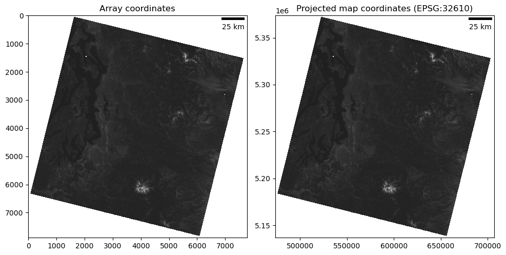
Add a dynamic scalebar to the above plot#
We will use the
matplotlib-scalebarpackage for thisSee documentation: https://github.com/ppinard/matplotlib-scalebar
The constructor arguments dx and units specify the pixel dimension. For example scalebar = ScaleBar(0.2, ‘um’) indicates that each pixel is equal to 0.2 micrometer. If the the axes image has already been calibrated by setting its extent, set dx to 1.0. * In other words: * For imshow using array coordinates (without defining
extent), useax.add_artist(ScaleBar(res))whereresis the pixel resolution in meters * For imshow using projected coordinates withextentdefined, useax.add_artist(ScaleBar(1.0))because one unit in the axes coordinate system is equal to 1 m
Note that you can control the location of the scalebar with the
locationkeyword argument, passed to theScaleBar()constructor: https://github.com/ppinard/matplotlib-scalebar#locationIf using interactive matplotlib backend, note what happens to the scalebar when you zoom
#Student Exercise
Part 5: Raster window extraction#
Review: array indexing#
We could continue our analysis with the full images, but for many science and engineering applications, we only care about a small subset of a raster at any given time
It’s also a good practice to prototype new workflows using a small subset of data
Less memory usage, much faster processing, faster debugging
Remember this for your project! Don’t start with full-resolution raster data.
One way to accomplish this might be to extract a portion of the large array using slicing/striding (see the Lab03 NumPy section)
Maybe a good time to review https://numpy.org/doc/stable/user/basics.indexing.html#slicing-and-striding
To extract a 1024x1024 px chunk of the full-size array, we could do something like:
r_sr.shape
(7891, 7771)
chunk = r_sr[3000:4024,3000:4024]
chunk.shape
(1024, 1024)
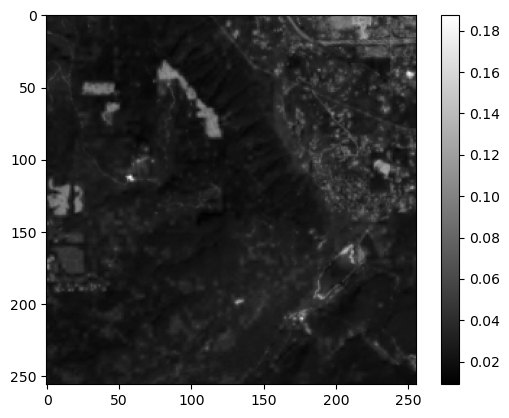
Extra Credit: extract a 256x256 pixel window around the center pixel of the array#
You already determined the center pixel indices earlier
You’ll need to define the appropriate slices for both rows and columns
Use variables to define window dimensions, rather than hardcoding 256 or 128
Preview the resulting 256x256 pixel array with imshow
#Student Exercise
#Student Exercise
Nice Job!#
Save this notebook, then
git addandgit commitShut down the kernel to free RAM
Proceed to Notebook #2!
We will explore the with rasterio
windowfunctionality to extract windows directly from the original tif files, then do all kinds of cool raster analysis with the resulting arrays
#Student Exercise