Vector 2: Geometries, Spatial Operations and Visualization Exercises
Contents
Vector 2: Geometries, Spatial Operations and Visualization Exercises#
UW Geospatial Data Analysis
CEE467/CEWA567
David Shean
Objectives#
Continue to explore GeoPandas functionality
Explore basic geometry operations (e.g., buffer, intersect, union)
Explore spatial filtering and spatial joins
Explore new visualization approaches (e.g., hexbin, interactive maps)
Let’s use the ICESat GLAS dataset one final time and cover some additional important vector concepts.
Part 0: Prepare data#
import matplotlib.pyplot as plt
import numpy as np
import pandas as pd
import geopandas as gpd
from shapely.geometry import Point, Polygon
import fiona
import xyzservices.providers as xyz
#plt.rcParams['figure.figsize'] = [10, 8]
Read in the projected GLAS points#
Ideally, use the exported gpkg file with equal-area projection from Lab04
Note, you can right-click on a file in the Jupyterlab file browser, and select “Copy Path”, then paste, but make sure you get the correct relative path to the current notebook (
../)If you have issues with your file, you can recreate:
Read the original GLAS csv
Load into GeoDataFrame, define CRS (
'EPSG:4326')Reproject with following PROJ string:
'+proj=aea +lat_1=37.00 +lat_2=47.00 +lat_0=42.00 +lon_0=-114.27'
#Loading from Lab04
#aea_fn = '../04_Vector1_Geopandas_CRS_Proj/conus_glas_aea.gpkg'
#glas_gdf_aea = gpd.read_file(aea_fn)
#Recreating
aea_proj_str = '+proj=aea +lat_1=37.00 +lat_2=47.00 +lat_0=42.00 +lon_0=-114.27'
csv_fn = '../01_Shell_Github/data/GLAH14_tllz_conus_lulcfilt_demfilt.csv'
glas_df = pd.read_csv(csv_fn)
glas_gdf = gpd.GeoDataFrame(glas_df, crs='EPSG:4326', geometry=gpd.points_from_xy(glas_df['lon'], glas_df['lat']))
glas_gdf_aea = glas_gdf.to_crs(aea_proj_str)
glas_gdf_aea.head()
| decyear | ordinal | lat | lon | glas_z | dem_z | dem_z_std | lulc | geometry | |
|---|---|---|---|---|---|---|---|---|---|
| 0 | 2003.139571 | 731266.943345 | 44.157897 | -105.356562 | 1398.51 | 1400.52 | 0.33 | 31 | POINT (709465.483 277418.898) |
| 1 | 2003.139571 | 731266.943346 | 44.150175 | -105.358116 | 1387.11 | 1384.64 | 0.43 | 31 | POINT (709431.326 276549.914) |
| 2 | 2003.139571 | 731266.943347 | 44.148632 | -105.358427 | 1392.83 | 1383.49 | 0.28 | 31 | POINT (709424.459 276376.270) |
| 3 | 2003.139571 | 731266.943347 | 44.147087 | -105.358738 | 1384.24 | 1382.85 | 0.84 | 31 | POINT (709417.614 276202.405) |
| 4 | 2003.139571 | 731266.943347 | 44.145542 | -105.359048 | 1369.21 | 1380.24 | 1.73 | 31 | POINT (709410.847 276028.547) |
Create a variable to store the crs of your GeoDataFrame#
Quickly print this out to verify everything looks good
aea_crs = glas_gdf_aea.crs
aea_crs
<Derived Projected CRS: +proj=aea +lat_1=37.00 +lat_2=47.00 +lat_0=42.00 + ...>
Name: unknown
Axis Info [cartesian]:
- E[east]: Easting (metre)
- N[north]: Northing (metre)
Area of Use:
- undefined
Coordinate Operation:
- name: unknown
- method: Albers Equal Area
Datum: World Geodetic System 1984
- Ellipsoid: WGS 84
- Prime Meridian: Greenwich
Read in the state polygons#
states_url = 'http://eric.clst.org/assets/wiki/uploads/Stuff/gz_2010_us_040_00_5m.json'
#states_url = 'http://eric.clst.org/assets/wiki/uploads/Stuff/gz_2010_us_040_00_500k.json'
states_gdf = gpd.read_file(states_url)
Limit to Lower48#
idx = states_gdf['NAME'].isin(['Alaska','Puerto Rico','Hawaii'])
states_gdf = states_gdf[~idx]
Reproject the states to match the crs of your points#
states_gdf_aea = states_gdf.to_crs(aea_crs)
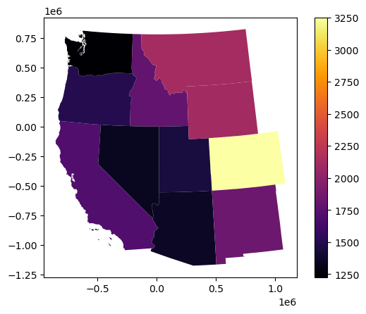
Create a quick plot to verify everything looks good#
Can re-use plotting code near the end of Lab04
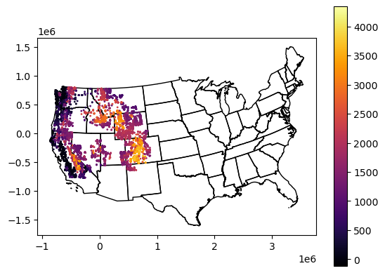
f, ax = plt.subplots()
states_gdf_aea.plot(ax=ax, facecolor='none', edgecolor='k')
glas_gdf_aea.plot(ax=ax, column='glas_z', cmap='inferno', markersize=1, legend=True);
Extract the MultiPolygon geometry object for Washington from your reprojected states GeoDataFrame#
Use the state ‘NAME’ value to isolate the approprate GeoDataFrame record for Washington
Assign the
geometryattribute for this record to a new variable calledwa_geomThis is a little tricky
After a boolean filter to get the WA record, you will need to use something like
iloc[0]to extract a GeoSeries, and then isolate thegeometryattributewa_geom = wa_gdf.iloc[0].geometry
Use the python
type()function to verify that your output type isshapely.geometry.multipolygon.MultiPolygon
# This is a new GeoDataFrame with one entry
wa_gdf = states_gdf_aea[states_gdf_aea['NAME'] == 'Washington']
# This is the Geometry object for that one entry
wa_geom = wa_gdf.squeeze().geometry
Find the geometric center of WA state#
See the
centroidattributeYou may have to
print()this to see the coordinates
#GeoDataFrame
#c = wa_gdf.centroid.iloc[0]
#MultiPolygon Geometry
c = wa_geom.centroid
c

Part 1: Geometric Operations for GLAS points#
Clip the GLAS points to Washington state polygon#
This should be pretty straightforward:
Identify records from the GLAS GeoDataFrame that
intersectsthe WA state geometryExtract those records and store in a new GeoDataFrame
This may take 5-10 seconds to complete
#Student Exercise
Compute some statistics for the WA state GLAS points#
How many points are in WA state?
What is mean
glas_zelevation in WA state?
#Student Exercise
5265
#Student Exercise
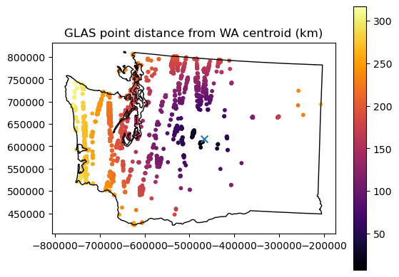
Plot the resulting points#
Add the WA polygon outline
Note that you don’t need/want to use the Polygon Geometry object here. Remember, you have a GeoDataFrame containing just the WA geometry. And you know how to plot GeoDataFrames.
Add the WA state centroid you calculated earlier using a distinct marker style (e.g.,
'*'or'x')Can use simple matplotlib
plotwith the coordinates, or can usewa_gdf.centroid.plot()
#Student Exercise
Find the GLAS point closest to the WA state centroid#
See the GeoDataFrame
distancefunctionCreate a plot showing this distance for each GLAS point.
#Student Exercise
#Student Exercise
What is the distance between this point and the centroid in km?#
#Student Exercise
Extra Credit: Do a quick calculation using the Pythagorean theorem to determine Euclidian distance between the centroid and this point - does this match the output of the
distancefunction?
What is the glas_z value of this point?#
For this, we need to isolate the original GeoDataFrame record corresponding to the minimum distance
We talked about
argminorargmaxfor NumPy arrays. For a DataFrame, we want to use theidxmin()method on the column or DataSeries containing the distance values, which should give us the index value:https://pandas.pydata.org/docs/reference/api/pandas.DataFrame.idxmin.html
Can then use the index value to locate the corresponding record in the GeoDataFrame with standard Pandas indexing: https://pandas.pydata.org/docs/user_guide/indexing.html
#Student Exercise
#Student Exercise
#Student Exercise
1539.35
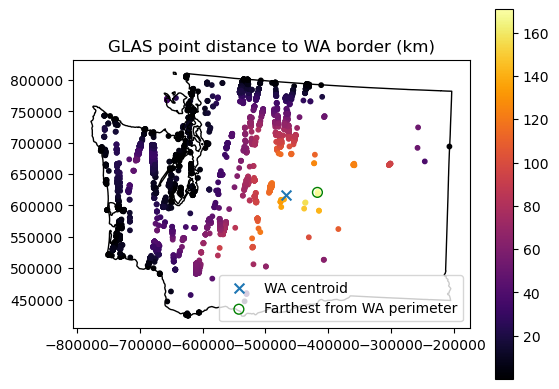
Extra Credit: Which GLAS point is farthest from the WA state perimeter?#
Note that this is different than the above calcuations for point to point distance, you’re looking for point to polyline distance
What is the distance in km?
This should be pretty straightforward, combining elements from the above questions/demo
This can be useful to consider distance from the coast and climatology (temperature, precipitation and other environmental variables)
#Student Exercise
#Student Exercise
#Student Exercise
Part 2: Aggregate GLAS points for state polygons and compute glas_z statistics#
OK, we computed some stats for GLAS points within WA state. Now let’s find the GLAS points that intersect each state polygon.
Objectives:
Compute the total number of points and mean
glas_zpoint elevation for each stateGenerate choropleth maps for both
One approach would be to loop through each state polygon, and do an intersection operation like we did for WA state above. But this is inefficient, and doesn’t scale well. It is much more efficient to do a spatial join between the points and the polygons with the intersection operator, then groupby and aggregate to compute the relevant statistics for each state.
You may have learned how to perform a join or spatial join in a GIS class. So, do we need to open ArcMap or QGIS here? Do we need a full-fledged spatial database like PostGIS? No! GeoPandas has you covered.
Start with a spatial join between the GLAS points and state polygons#
Start by reviewing the Spatial Join documentation here: http://geopandas.org/mergingdata.html
Use the geopandas
sjoinmethod: http://geopandas.org/reference/geopandas.sjoin.html
Let’s extract the columns that matter#
Since we only care about
glas_zvalues here let’s create some smaller GeoDataFrames:Extract the
['glas_z', 'geometry']columns from the GLAS GeoDataFrameExtract the
['NAME', 'geometry']columns from the states GeoDataFrame
glas_gdf_aea_lite = glas_gdf_aea[['glas_z', 'geometry']]
states_gdf_aea_lite = states_gdf_aea[['NAME','geometry']]
Now try a spatial join between these two#
Use the GLAS points as the “left” GeoDataFrame and the States as the “right” GeoDataFrame
Start by using default options (
op='intersects', how='inner')Note the output geometry type and columns
#Student Exercise
| glas_z | geometry | index_right | NAME | |
|---|---|---|---|---|
| 0 | 1398.51 | POINT (709465.483 277418.898) | 50 | Wyoming |
| 1 | 1387.11 | POINT (709431.326 276549.914) | 50 | Wyoming |
| 2 | 1392.83 | POINT (709424.459 276376.270) | 50 | Wyoming |
| 3 | 1384.24 | POINT (709417.614 276202.405) | 50 | Wyoming |
| 4 | 1369.21 | POINT (709410.847 276028.547) | 50 | Wyoming |
| ... | ... | ... | ... | ... |
| 64091 | 1868.30 | POINT (485179.859 -614501.598) | 31 | New Mexico |
| 64499 | 1701.32 | POINT (531778.415 -627890.213) | 31 | New Mexico |
| 64500 | 1735.44 | POINT (531666.256 -629442.175) | 31 | New Mexico |
| 8377 | 1362.41 | POINT (87991.625 -555886.651) | 2 | Arizona |
| 60425 | 1348.03 | POINT (87811.448 -556041.104) | 2 | Arizona |
63850 rows × 4 columns
Now reverse the order of the two input GeoDataFrames#
Use default options again
#Student Exercise
Which one makes more sense?#
Remember, we’re trying to add a State name to each GLAS point
You’ll need to decide which one to use moving forward
#Student Exercise
Extra credit#
Experiment with a few different operations (op) for the spatial join (e.g., intersects) and review the output with head()
Descriptions of different operations are here: https://shapely.readthedocs.io/en/stable/manual.html#object.intersects
Note that for our input spatial join of points and polygons, some of the details are irrelevant
Do you notice a difference in the output number of records?
Choose the
howkeyword appropriately:Test a few options and note the output number of records
Are there any points that don’t fall within a state polygon? Why might this be? Do you want to preserve these moving forward?
#Student Exercise
Sanity check#
Run a
headon our new GeoDataFrameFor each GLAS point, there should be a new column with the corresponding state NAME
Check the original and joined
shapeDoes the number of records equal the original number of GLAS points?
Why might they be different?
Extra credit: plot the points that were not included in spatial join#
Does the spatial distribution help you answer the above question?
Maybe useful to zoom in to look at points and state outlines
#Student Exercise
| glas_z | geometry | index_right | NAME | |
|---|---|---|---|---|
| 0 | 1398.51 | POINT (709465.483 277418.898) | 50 | Wyoming |
| 1 | 1387.11 | POINT (709431.326 276549.914) | 50 | Wyoming |
| 2 | 1392.83 | POINT (709424.459 276376.270) | 50 | Wyoming |
| 3 | 1384.24 | POINT (709417.614 276202.405) | 50 | Wyoming |
| 4 | 1369.21 | POINT (709410.847 276028.547) | 50 | Wyoming |
#Student Exercise
Original count: 65236
Joined count: 63850
#Student Exercise
#Student Exercise
Now aggregate by state NAME#
Note: the GeoPandas doc example uses a
dissolveoperation here, which is a wrapper around thegroupbyandaggPandas functionsBut look at the geometry column for the points in your GeoDataFrame. The
dissolveis going to compute the union for the points in each state and return aMultiPointGeometry for each state, which we don’t really want/need. It will also take longer to run.Instead, let’s try a
groupbyoperation for theNAMEcolumn, and thenaggwith a list of functions we care about:['count', 'mean'](statitiscs for point count and mean point elevation for each state)
#Student Exercise
/tmp/ipykernel_465/4031457243.py:2: FutureWarning: ['geometry'] did not aggregate successfully. If any error is raised this will raise in a future version of pandas. Drop these columns/ops to avoid this warning.
  glas_gdf_aea_states_agg = glas_gdf_aea_states.groupby('NAME').agg(['count', 'mean'])
| glas_z | index_right | |||
|---|---|---|---|---|
| count | mean | count | mean | |
| NAME | ||||
| Arizona | 2 | 1355.220000 | 2 | 2.0 |
| California | 13865 | 1701.699116 | 13865 | 4.0 |
| Colorado | 8429 | 3253.791521 | 8429 | 5.0 |
| Idaho | 7297 | 1790.290550 | 7297 | 12.0 |
| Montana | 2658 | 2125.944759 | 2658 | 26.0 |
| Nevada | 12081 | 1335.431521 | 12081 | 28.0 |
| New Mexico | 209 | 1835.156699 | 209 | 31.0 |
| Oregon | 2838 | 1500.335525 | 2838 | 37.0 |
| Utah | 5498 | 1439.914989 | 5498 | 44.0 |
| Washington | 5265 | 1224.196596 | 5265 | 47.0 |
| Wyoming | 5708 | 2106.420340 | 5708 | 50.0 |
Sanity check#
That groupby and agg should be pretty fast (~1-2 seconds)
Check the
type()of the outputSince
groupbyandaggare Pandas operation, you should now have a new PandasDataFrame(not a GeoPandasGeoDataFrame) with index of state names and columns forcountandmeanvalues in each state
#Student Exercise
Simplify the Heirarchical Index#
However, you may have noticed that you now have a “heirarchical index”, with
countandmeancolumns for bothglas_zandindex_right.More info on this is here: https://pandas.pydata.org/pandas-docs/stable/user_guide/advanced.html
This can be confusing at first, but is actually a powerful feature of Pandas.
For our situation, we don’t care about
index_right(byproduct of our spatial join), so you can simplify by extracting only theglas_zvaluesDo this the way you would extract a column from a standard DataFrame:
my_agg_df['glas_z']and store as a new DataFrameYou can now directly access the
countandmeancolumns
#Student Exercise
Part 3: Plots!#
How are we going to visualize these data?
We have
countandmeanof GLAS points for each state! Objective #1 complete!We now want to visualize these values, but we lost our state Polygon/MultiPolygon Geometry along the way
No problem, we can combine our DataFrame with the original State GeoDataFrame
Can use
mergeto do an attribute join on the shared state'NAME'index for the twoTake a moment to review the
my_agg_df.merge?optionsIn this case, we have a common
NAMEfield, so we can use theon='NAME'here for attribute join
Careful about the order of the two inputs here (state GeoDataFrame and the DataFrame with your stats) - you want to preserve the index and geometry of the GeoDataFrame, adding the
countandmeancolumns.If you get it right, you should be able to
plot()the GeoPandas GeoDataFrame and get a map. If you got it backwards, the output ofplot()will be a line plot for the regular Pandas DataFrame
#Student Exercise
| NAME | geometry | count | mean | |
|---|---|---|---|---|
| 0 | Arizona | POLYGON ((154103.502 -554865.569, 154463.722 -... | 2 | 1355.220000 |
| 1 | California | MULTIPOLYGON (((-715337.404 -425936.004, -7153... | 13865 | 1701.699116 |
| 2 | Colorado | POLYGON ((676361.242 -79930.861, 687165.323 -7... | 8429 | 3253.791521 |
| 3 | Idaho | POLYGON ((261921.702 118654.345, 261929.542 11... | 7297 | 1790.290550 |
| 4 | Montana | POLYGON ((724628.849 373437.826, 721641.649 37... | 2658 | 2125.944759 |
| 5 | Nevada | POLYGON ((19102.023 -111459.675, 19082.720 -13... | 12081 | 1335.431521 |
| 6 | New Mexico | POLYGON ((788203.103 -1070451.319, 778535.190 ... | 209 | 1835.156699 |
| 7 | Oregon | POLYGON ((-594594.782 433232.266, -593459.687 ... | 2838 | 1500.335525 |
| 8 | Utah | POLYGON ((269119.721 -78373.504, 270165.794 -1... | 5498 | 1439.914989 |
| 9 | Washington | MULTIPOLYGON (((-612752.940 729560.713, -61302... | 5265 | 1224.196596 |
| 10 | Wyoming | POLYGON ((353778.866 -103059.499, 347654.788 -... | 5708 | 2106.420340 |
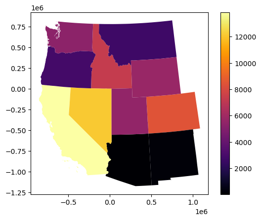
Create a choropleth map to visualize the count of GLAS points in each state#
#Student Exercise
Create a choropleth map to visualize the mean elevation GLAS points in each state#
#Student Exercise
Part 4: Point Densitiy Visualization: Hexbin plots#
OK, now we have statistics and plots for our existing polygons. But what if we want to compute similar statistics for a regularly spaced grid of cells? For our count, this will give us point density, allowing for better visualization of the spatial distribution.
We could define a set of adjacent rectangular polygons, and repeat our sjoin, groupby, agg sequence above. Or we can use some existing matplotlib functionality, and create a hexbin plot!
Hexagonal cells are preferable over a standard square/rectangular grid for various reasons: https://pro.arcgis.com/en/pro-app/tool-reference/spatial-statistics/h-whyhexagons.htm
Side note: Sarah Battersby (Tableau) had a nice paper exploring these issues for different projections: https://www.tandfonline.com/doi/full/10.1080/15230406.2016.1180263. “Shapes on a plane” is one of the better journal article titles I’ve ever seen :).
Here are some resources on generating hexbins using Python and matplotlib:
Note: an equal-area projection is always good idea for a hexbin plot. Fortunately, we started with our AEA projection, so we’re all set!
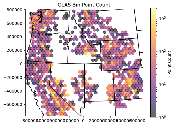
Create a hexbin that shows the number of points in each cell#
Play around with the
gridsizeoption to set the number of bins in each dimension (or specify the dimensions of your bins)Use the
mincntoption to avoid plotting cells with 0 countOverlay the state polygons to help visualize
Set your plot
xlimandylimto the GLAS point boundsCan use linear color ramp with vmin and vmax options, or try a logarithmic color ramp, since we have a broad range of counts
#Student Exercise
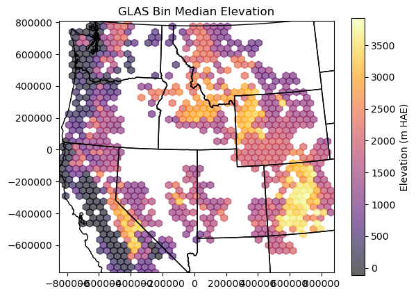
Create a second hexbin plot that shows the median elevation in each cell#
See documentation for the
Candreduce_C_functionoptions
#Student Exercise
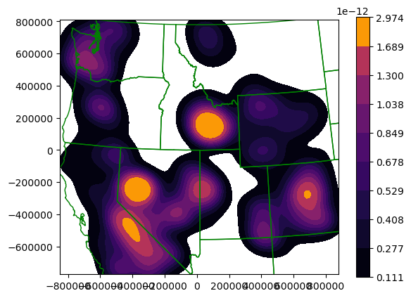
Extra Credit: Generate a Kernel Density Estimator (KDE) plot using seaborn#
This is another nice approach to estimate the point density on a continuous grid
See motivation here for an explanation: https://en.wikipedia.org/wiki/Multivariate_kernel_density_estimation#Motivation
Seaborn has a nice implementation for 2D data
glas_gdf_aea['glas_z'].values
array([1398.51, 1387.11, 1392.83, ..., 1556.19, 1556.18, 1556.32])
#Student Exercise
Static plots with tiled basemaps using contextily#
Our state outlines provide some context for our plots, but what if we want a raster map background
Can use the convenientt
contextilypackage for this: https://github.com/geopandas/contextily
import contextily as ctx
ctx.providers.Stamen.Terrain
- url
- https://stamen-tiles-{s}.a.ssl.fastly.net/{variant}/{z}/{x}/{y}{r}.{ext}
- html_attribution
- Map tiles by Stamen Design, CC BY 3.0 — Map data © OpenStreetMap contributors
- attribution
- Map tiles by Stamen Design, CC BY 3.0 -- Map data (C) OpenStreetMap contributors
- subdomains
- abcd
- min_zoom
- 0
- max_zoom
- 18
- variant
- terrain
- ext
- png
Using the default basemap projection#
Freely available tiled web maps are great: https://en.wikipedia.org/wiki/Tiled_web_map
Most tiled basemaps use a standard “web mercator” projection (EPSG:3857)
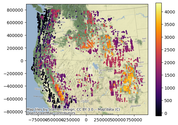
For this example, we will reproject our point GeoDataFrame to match the default tiles
f, ax = plt.subplots()
#Convert points to web mercator projection and plot
glas_gdf_aea.to_crs('EPSG:3857').plot(ax=ax, column='glas_z', cmap='inferno', markersize=2, legend=True)
#Add basemap
ctx.add_basemap(ax=ax, source=ctx.providers.Stamen.Terrain)
Plot the WA points#
Explore different zoom levels
Try at least one additional different ctx.provider
Maybe
ctx.providers.Esri.WorldImagery
#Student Exercise
Using our custom projected coordinate system#
The contextily package also supports simple tile warping into arbitrary projections: https://contextily.readthedocs.io/en/latest/warping_guide.html
Note the
add_basemapcall is similar, just need to pass in the appropriate CRS object
We will revisit raster reprojection during the Raster 2 lab, but for now try to plot using the Albers Equal-area projection
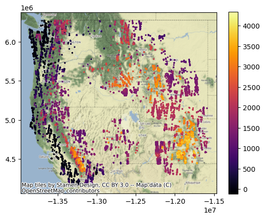
Note the curvature of the 49° parallel (border between US and Canada) compared to earlier plot in web mercator projection
f, ax = plt.subplots()
#Convert points to web mercator projection and plot
glas_gdf_aea.plot(ax=ax, column='glas_z', cmap='inferno', markersize=2, legend=True)
#Add basemap, specifying crs keyword
ctx.add_basemap(ax=ax, crs=glas_gdf_aea.crs, source=ctx.providers.Stamen.Terrain)
Repeat for WA state#
#Student Exercise
Part 5: Interactive plots#
See standalone notebook
Extra Credit#
Create a function to identify the 3 closest points to each GLAS point#
Then use these 3 points to:
Define a plane
Calculate the elevation on that planar surface at the original GLAS point coordinates
Compute the difference between the observed GLAS elevation and the interpolated elevation
For each GLAS point, compute mean and std for all points within a 10 km radius#
Can potentially create buffer around the point, then intersect with all points
Can compute distance to all points, then threshold
Load the Randolph Glacier Inventory polygons (see demo) and do a spatial join with state polygons#
Compute and plot the number of glaciers and total glacier area within each state.
Which state has the highest number and area?