Demo: Landsat and Dynamic Data Access
Contents
Demo: Landsat and Dynamic Data Access#
UW Geospatial Data Analysis
CEE467/CEWA567
David Shean
Introduction#
Hopefully you’ve all seen or used Landsat imagery at some point in the past
Take a few minutes to refresh your memory: https://www.usgs.gov/land-resources/nli/landsat
There is a huge amount of information out there on the Landsat missions, data products, science results
USGS and NASA partnership
Landsat-8#
Landsat-8 is the mission (a satellite)
Operational Land Imager (OLI) is an instrument (a camera)
Thermal Infrared Sensor (TIRS) is an insitrument (also a camera, but measures thermal infrared radiation, surface temperature)
Take a look at useful info here:
Orbit and Data collection#
Landsat 8 orbits the the Earth in a sun-synchronous, near-polar orbit, at an altitude of 705 km (438 mi), inclined at 98.2 degrees, and completes one Earth orbit every 99 minutes. The satellite has a 16-day repeat cycle with an equatorial crossing time: 10:00 a.m. +/- 15 minutes.
Landsat 8 aquires about 740 scenes a day on the Worldwide Reference System-2 (WRS-2) path/row system, with a swath overlap (or sidelap) varying from 7 percent at the equator to a maximum of approximately 85 percent at extreme latitudes. A Landsat 8 scene size is 185 km x 180 km (114 mi x 112 mi).
Instruments and Bands#
So, Landsat-8 sensor is the top row of colored bands in the following figure (lower rows are for older Landsat sensors):
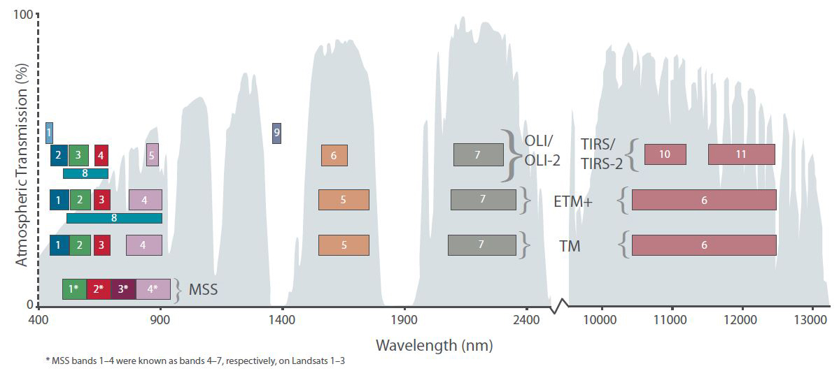
For comparison with previous Landsat missions: https://www.usgs.gov/faqs/what-are-band-designations-landsat-satellites?qt-news_science_products=0#qt-news_science_products
Dynamic Range#
LS8 OLI provides 12-bit dynamic range, which improves signal to noise ratio.
Remember, each bit is a 0 or 1. We have 12 of them, so we have 2^12 (or 4096) unique combinations to represent brightness in the image.
Most data types on a computer are in multiples of bytes, which have 8 bits. For example, a typical RGB image of a cat face contains three 8-bit channels for red, green and blue values.
LS8 offers a considerable improvement over for the 8-bit dynamic range of Landsat 1-7. Improved signal to noise performance enables improved characterization of land cover state and condition.
We don’t have a convenient mechanism to store 12-bit data, so the LS8 images are stored as 16-bit unsigned integers (2^16 possible values, 0-65535)
The initial values (spanning 0-4095) are scaled across 55000 of the total 65535 brightness levels in the 16-bit images
Image Resolution - Ground Sample Distance (GSD)#
Panchromatic (PAN) band (band number 8) has 15 m ground sample distance (GSD)
Multispectral (MS) bands are 30 m GSD
Thermal IR are 100 m GSD, but are often oversampled to match MS bands
Landsat-8 Data Products#
The standard data products are “Level 1” images: they radiometrically corrected and orthorectified (terrain corrected) in the approprate UTM projection: https://www.usgs.gov/core-science-systems/nli/landsat/landsat-level-1-processing-details
For more sophisticated analysis, you typically want to use higher-level, calibrated/corrected products (“level 2” like surface reflectance values), often considered “Analysis Ready Data (ARD)”: https://www.usgs.gov/land-resources/nli/landsat/landsat-science-products
Information about Digital Number (DN), top of atmosphere (TOA) and surface reflectance (SR): https://www.l3harrisgeospatial.com/Learn/Blogs/Blog-Details/ArtMID/10198/ArticleID/16278/Digital-Number-Radiance-and-Reflectance
Top of Atmosphere reflectance
Formulas for conversion of DN to TOA: https://www.usgs.gov/landsat-missions/using-usgs-landsat-level-1-data-product
“Surface reflectance is the amount of light reflected by the surface of the Earth. It is a ratio of surface radiance to surface irradiance, and as such is unitless, with values between 0 and 1.”
“Surface reflectance (SR) improves comparison between multiple images over the same region by accounting for atmospheric effects such as aerosol scattering and thin clouds, which can help in the detection and characterization of Earth surface change. “
“Landsat 8 OLI Collection 1 Surface Reflectance are generated using the Land Surface Reflectance Code (LaSRC) (version 1.4.1), which makes use of the coastal aerosol band to perform aerosol inversion tests, uses auxiliary climate data from MODIS, and uses a unique radiative transfer model. (Vermote et al., 2016).”
Path/Row system#
https://landsat.gsfc.nasa.gov/the-worldwide-reference-system/
Use descending for daytime imagery
Seattle and Mt. Rainier: path 46, row 27
LS8 Data availability#
USGS/NASA hosts the official Landsat products. This option is great for one-off interactive data searches, but can be clunky and requires a lot of manual steps:
Commercial cloud providers now mirror the entire USGS archive, and provide a much more efficient API (application programming interface) to access the data. This is especially important when you need to access 100s-1000s of images.
Google:
Amazon Web Services (AWS):
Microsoft Planetary Computer:
Finding cloud-free imagery#
The process of identifying and downloading data has evolved considerably throughout the Landsat missions, and modern approaches use on-demand access to cloud-hosted archives, often without local downloads.
Interactive, manual approach: use EarthExplorer for visual queries: https://earthexplorer.usgs.gov/
Get the image ID
Can also directly download products from EarthExplorer, but pretty inefficient
Automated, programmatic approach: query archives from Python API or command-line, using SpatioTemporal Asset Catalog (STAC): https://landsat.stac.cloud
Other approaches: https://www.usgs.gov/landsat-missions/landsat-data-access
For now, let’s use some code to download some pre-identified images for WA state to the hub. Note that we could do all of this on the fly, but for experimentation and development, having a local copy of sample images will speed up reading.
import os
import urllib
import rasterio as rio
import rasterio.plot
import requests
Note that we can open an image directly from a url#
(look Ma, no downloads!)
Let’s use the last url from our earlier download as a test
image_url = 'https://storage.googleapis.com/gcp-public-data-landsat/LC08/01/046/027/LC08_L1TP_046027_20180818_20180829_01_T1/LC08_L1TP_046027_20180818_20180829_01_T1_B10.TIF'
print(image_url)
https://storage.googleapis.com/gcp-public-data-landsat/LC08/01/046/027/LC08_L1TP_046027_20180818_20180829_01_T1/LC08_L1TP_046027_20180818_20180829_01_T1_B10.TIF
src = rio.open(image_url)
src.profile
{'driver': 'GTiff', 'dtype': 'uint16', 'nodata': None, 'width': 7781, 'height': 7881, 'count': 1, 'crs': CRS.from_epsg(32610), 'transform': Affine(30.0, 0.0, 473385.0,
       0.0, -30.0, 5373315.0), 'blockxsize': 256, 'blockysize': 256, 'tiled': True, 'compress': 'lzw', 'interleave': 'band'}
with rio.open(image_url) as src:
    print(src.profile)
{'driver': 'GTiff', 'dtype': 'uint16', 'nodata': None, 'width': 7781, 'height': 7881, 'count': 1, 'crs': CRS.from_epsg(32610), 'transform': Affine(30.0, 0.0, 473385.0,
       0.0, -30.0, 5373315.0), 'blockxsize': 256, 'blockysize': 256, 'tiled': True, 'compress': 'lzw', 'interleave': 'band'}
#Note that the dataset does not remain open!
src
<closed DatasetReader name='https://storage.googleapis.com/gcp-public-data-landsat/LC08/01/046/027/LC08_L1TP_046027_20180818_20180829_01_T1/LC08_L1TP_046027_20180818_20180829_01_T1_B10.TIF' mode='r'>
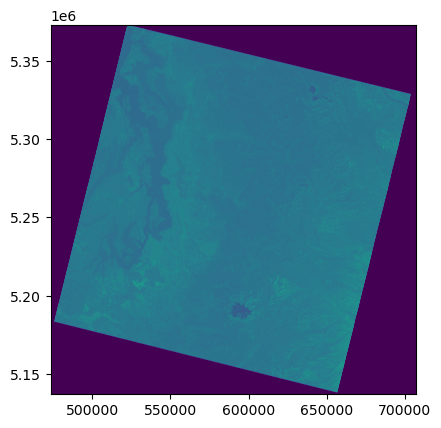
with rio.open(image_url) as src:
    rio.plot.show(src)
Download Collection 2 (L2) products for Surface Reflectance and Surface Temperature#
#Create local directory to store images
imgdir = 'LS8_sample'
if not os.path.exists(imgdir):
    os.makedirs(imgdir)
Download assets for specific images#
Dynamimcally construct url using known information
Using Microsoft Planetary Computer archive of Collection 2 Level 2 images
Need to obtain token to authenticate (“sign”) urls
#Collection name
collection = 'landsat-8-c2-l2'
#Base url for this collection
base_url = 'https://landsateuwest.blob.core.windows.net/landsat-c2/level-2/standard/oli-tirs'
#List of predetermined images (e.g., from STAC, or interactive EarthExplorer or EarthData search)
img_list = ['LC08_L2SP_046027_20180818_20200831_02_T1', \
            'LC08_L2SP_046027_20181224_20200829_02_T1']
#Subset of assets to download (specific bands for L2 surface reflectance/temperature products)
#Note: no panchromatic (B8) avialable from this collection
asset_id_list = ['SR_B1', 'SR_B2', 'SR_B3', 'SR_B4', 'SR_B5', 'SR_B6', 'SR_B7', 'ST_B10', 'reduced_resolution_browse']
Notes on LS filenames:
# Get a token for signed url preparation
resp = requests.get(f'https://planetarycomputer.microsoft.com/api/sas/v1/token/{collection}')
token = resp.json()['token']
#Loop through all selected images and all bands
for img in img_list:
    for asset_id in asset_id_list:
        #Generate the appropriate URL for the image IDs
        year = img.split('_')[3][0:4]
        path = img.split('_')[2][0:3]
        row = img.split('_')[2][3:]
        if asset_id == 'reduced_resolution_browse':
            image_url =  f'{base_url}/{year}/{path}/{row}/{img}/{img}_thumb_large.jpeg'
        else:
            image_url =  f'{base_url}/{year}/{path}/{row}/{img}/{img}_{asset_id}.TIF'
            #image_url =  f'{base_url}/{year}/{path:03d}/{row:03d}/{img}/{img}_{asset_id}.TIF'
        print(f'{image_url}?{token}')
        #Local filename
        out_fn = os.path.join(imgdir, os.path.split(image_url)[-1])
        #Check to see if file already exists
        if not os.path.exists(out_fn):
            #signed_asset = pc.sign_asset(pystac.asset.Asset(image_url))
            print("Saving:", out_fn)
            #Download the file
            urllib.request.urlretrieve(f'{image_url}?{token}', out_fn)
Do a quick ls -lh on the local image directory#
Note relative file sizes for the different bands of each image
B8 vs B3 vs. B10
Revisit the chart above - does this make sense for resolution of these bands?
!ls -lh $imgdir
total 1.9G
-rw-rw-r-- 1 jovyan users 257M Feb  3 03:57 LC08_L1TP_046027_20180818_20180829_01_T1_B8.TIF
-rw-rw-r-- 1 jovyan users 265M Feb  3 03:57 LC08_L1TP_046027_20181224_20190129_01_T1_B8.TIF
-rw-rw-r-- 1 jovyan users  81M Feb  1 04:02 LC08_L2SP_046027_20180818_20200831_02_T1_SR_B1.TIF
-rw-rw-r-- 1 jovyan users  81M Feb  1 04:02 LC08_L2SP_046027_20180818_20200831_02_T1_SR_B2.TIF
-rw-rw-r-- 1 jovyan users  82M Feb  1 04:02 LC08_L2SP_046027_20180818_20200831_02_T1_SR_B3.TIF
-rw-rw-r-- 1 jovyan users  83M Feb  1 04:03 LC08_L2SP_046027_20180818_20200831_02_T1_SR_B4.TIF
-rw-rw-r-- 1 jovyan users  92M Feb  1 04:03 LC08_L2SP_046027_20180818_20200831_02_T1_SR_B5.TIF
-rw-rw-r-- 1 jovyan users  90M Feb  1 04:03 LC08_L2SP_046027_20180818_20200831_02_T1_SR_B6.TIF
-rw-rw-r-- 1 jovyan users  86M Feb  1 04:03 LC08_L2SP_046027_20180818_20200831_02_T1_SR_B7.TIF
-rw-rw-r-- 1 jovyan users  84M Feb  1 19:20 LC08_L2SP_046027_20180818_20200831_02_T1_ST_B10.TIF
-rw-rw-r-- 1 jovyan users  89K Feb  1 04:04 LC08_L2SP_046027_20180818_20200831_02_T1_thumb_large.jpeg
-rw-rw-r-- 1 jovyan users  91M Feb  1 04:04 LC08_L2SP_046027_20181224_20200829_02_T1_SR_B1.TIF
-rw-rw-r-- 1 jovyan users  91M Feb  1 04:04 LC08_L2SP_046027_20181224_20200829_02_T1_SR_B2.TIF
-rw-rw-r-- 1 jovyan users  92M Feb  1 04:04 LC08_L2SP_046027_20181224_20200829_02_T1_SR_B3.TIF
-rw-rw-r-- 1 jovyan users  91M Feb  1 04:05 LC08_L2SP_046027_20181224_20200829_02_T1_SR_B4.TIF
-rw-rw-r-- 1 jovyan users  96M Feb  1 04:05 LC08_L2SP_046027_20181224_20200829_02_T1_SR_B5.TIF
-rw-rw-r-- 1 jovyan users  90M Feb  1 04:05 LC08_L2SP_046027_20181224_20200829_02_T1_SR_B6.TIF
-rw-rw-r-- 1 jovyan users  87M Feb  1 04:05 LC08_L2SP_046027_20181224_20200829_02_T1_SR_B7.TIF
-rw-rw-r-- 1 jovyan users  77M Feb  1 04:06 LC08_L2SP_046027_20181224_20200829_02_T1_ST_B10.TIF
-rw-rw-r-- 1 jovyan users  366 Feb  1 04:08 LC08_L2SP_046027_20181224_20200829_02_T1_ST_B10.TIF.aux.xml
-rw-r--r-- 1 jovyan users 155K Mar 11 21:42 LC08_L2SP_046027_20181224_20200829_02_T1_thumb_large.jpeg
Use gdalinfo command to get some basic information about one of the files#
Review output with your neighbor/group
🤔 Talk about what each line means, if there is something you don’t understand, ask! Or look it up together!
sample_fn = os.path.join(imgdir, img+'_ST_B10.TIF')
print(sample_fn)
LS8_sample/LC08_L2SP_046027_20181224_20200829_02_T1_ST_B10.TIF
!gdalinfo $sample_fn
Driver: GTiff/GeoTIFF
Files: LS8_sample/LC08_L2SP_046027_20181224_20200829_02_T1_ST_B10.TIF
       LS8_sample/LC08_L2SP_046027_20181224_20200829_02_T1_ST_B10.TIF.aux.xml
Size is 7771, 7881
Coordinate System is:
PROJCRS["WGS 84 / UTM zone 10N",
    BASEGEOGCRS["WGS 84",
        DATUM["World Geodetic System 1984",
            ELLIPSOID["WGS 84",6378137,298.257223563,
                LENGTHUNIT["metre",1]]],
        PRIMEM["Greenwich",0,
            ANGLEUNIT["degree",0.0174532925199433]],
        ID["EPSG",4326]],
    CONVERSION["UTM zone 10N",
        METHOD["Transverse Mercator",
            ID["EPSG",9807]],
        PARAMETER["Latitude of natural origin",0,
            ANGLEUNIT["degree",0.0174532925199433],
            ID["EPSG",8801]],
        PARAMETER["Longitude of natural origin",-123,
            ANGLEUNIT["degree",0.0174532925199433],
            ID["EPSG",8802]],
        PARAMETER["Scale factor at natural origin",0.9996,
            SCALEUNIT["unity",1],
            ID["EPSG",8805]],
        PARAMETER["False easting",500000,
            LENGTHUNIT["metre",1],
            ID["EPSG",8806]],
        PARAMETER["False northing",0,
            LENGTHUNIT["metre",1],
            ID["EPSG",8807]]],
    CS[Cartesian,2],
        AXIS["(E)",east,
            ORDER[1],
            LENGTHUNIT["metre",1]],
        AXIS["(N)",north,
            ORDER[2],
            LENGTHUNIT["metre",1]],
    USAGE[
        SCOPE["Engineering survey, topographic mapping."],
        AREA["Between 126°W and 120°W, northern hemisphere between equator and 84°N, onshore and offshore. Canada - British Columbia (BC); Northwest Territories (NWT); Nunavut; Yukon. United States (USA) - Alaska (AK)."],
        BBOX[0,-126,84,-120]],
    ID["EPSG",32610]]
Data axis to CRS axis mapping: 1,2
Origin = (472785.000000000000000,5373315.000000000000000)
Pixel Size = (30.000000000000000,-30.000000000000000)
Metadata:
  AREA_OR_POINT=Point
Image Structure Metadata:
  COMPRESSION=DEFLATE
  INTERLEAVE=BAND
Corner Coordinates:
Upper Left  (  472785.000, 5373315.000) (123d22' 6.59"W, 48d30'44.50"N)
Lower Left  (  472785.000, 5136885.000) (123d21'14.15"W, 46d23' 5.97"N)
Upper Right (  705915.000, 5373315.000) (120d12'48.76"W, 48d28'45.16"N)
Lower Right (  705915.000, 5136885.000) (120d19'24.73"W, 46d21'15.14"N)
Center      (  589350.000, 5255100.000) (121d48'53.62"W, 47d26'35.59"N)
Band 1 Block=256x256 Type=UInt16, ColorInterp=Gray
  Min=23752.000 Max=42219.000
  Minimum=23752.000, Maximum=42219.000, Mean=35708.987, StdDev=2100.959
  NoData Value=0
  Overviews: 3886x3941, 1943x1971, 972x986, 486x493, 243x247, 122x124
  Metadata:
    STATISTICS_MAXIMUM=42219
    STATISTICS_MEAN=35708.986610756
    STATISTICS_MINIMUM=23752
    STATISTICS_STDDEV=2100.9585113563
    STATISTICS_VALID_PERCENT=66.34
!gdalinfo $sample_fn -stats
Driver: GTiff/GeoTIFF
Files: LS8_sample/LC08_L2SP_046027_20181224_20200829_02_T1_ST_B10.TIF
       LS8_sample/LC08_L2SP_046027_20181224_20200829_02_T1_ST_B10.TIF.aux.xml
Size is 7771, 7881
Coordinate System is:
PROJCRS["WGS 84 / UTM zone 10N",
    BASEGEOGCRS["WGS 84",
        DATUM["World Geodetic System 1984",
            ELLIPSOID["WGS 84",6378137,298.257223563,
                LENGTHUNIT["metre",1]]],
        PRIMEM["Greenwich",0,
            ANGLEUNIT["degree",0.0174532925199433]],
        ID["EPSG",4326]],
    CONVERSION["UTM zone 10N",
        METHOD["Transverse Mercator",
            ID["EPSG",9807]],
        PARAMETER["Latitude of natural origin",0,
            ANGLEUNIT["degree",0.0174532925199433],
            ID["EPSG",8801]],
        PARAMETER["Longitude of natural origin",-123,
            ANGLEUNIT["degree",0.0174532925199433],
            ID["EPSG",8802]],
        PARAMETER["Scale factor at natural origin",0.9996,
            SCALEUNIT["unity",1],
            ID["EPSG",8805]],
        PARAMETER["False easting",500000,
            LENGTHUNIT["metre",1],
            ID["EPSG",8806]],
        PARAMETER["False northing",0,
            LENGTHUNIT["metre",1],
            ID["EPSG",8807]]],
    CS[Cartesian,2],
        AXIS["(E)",east,
            ORDER[1],
            LENGTHUNIT["metre",1]],
        AXIS["(N)",north,
            ORDER[2],
            LENGTHUNIT["metre",1]],
    USAGE[
        SCOPE["Engineering survey, topographic mapping."],
        AREA["Between 126°W and 120°W, northern hemisphere between equator and 84°N, onshore and offshore. Canada - British Columbia (BC); Northwest Territories (NWT); Nunavut; Yukon. United States (USA) - Alaska (AK)."],
        BBOX[0,-126,84,-120]],
    ID["EPSG",32610]]
Data axis to CRS axis mapping: 1,2
Origin = (472785.000000000000000,5373315.000000000000000)
Pixel Size = (30.000000000000000,-30.000000000000000)
Metadata:
  AREA_OR_POINT=Point
Image Structure Metadata:
  COMPRESSION=DEFLATE
  INTERLEAVE=BAND
Corner Coordinates:
Upper Left  (  472785.000, 5373315.000) (123d22' 6.59"W, 48d30'44.50"N)
Lower Left  (  472785.000, 5136885.000) (123d21'14.15"W, 46d23' 5.97"N)
Upper Right (  705915.000, 5373315.000) (120d12'48.76"W, 48d28'45.16"N)
Lower Right (  705915.000, 5136885.000) (120d19'24.73"W, 46d21'15.14"N)
Center      (  589350.000, 5255100.000) (121d48'53.62"W, 47d26'35.59"N)
Band 1 Block=256x256 Type=UInt16, ColorInterp=Gray
  Min=23752.000 Max=42219.000
  Minimum=23752.000, Maximum=42219.000, Mean=35708.987, StdDev=2100.959
  NoData Value=0
  Overviews: 3886x3941, 1943x1971, 972x986, 486x493, 243x247, 122x124
  Metadata:
    STATISTICS_MAXIMUM=42219
    STATISTICS_MEAN=35708.986610756
    STATISTICS_MINIMUM=23752
    STATISTICS_STDDEV=2100.9585113563
    STATISTICS_VALID_PERCENT=66.34
Other examples#
Catalog search with STAC#
This should be used when you don’t know image IDs up front
Can search with spatial and temporal limits
Set cell type as raw for now, since we know Image IDs
#Install necessary packages
#https://jakevdp.github.io/blog/2017/12/05/installing-python-packages-from-jupyter/
!mamba install --yes pystac planetary-computer
# Landsat-8 collection 2 from planetary computer
# https://planetarycomputer.microsoft.com/dataset/landsat-8-c2-l2#Example-Notebook

import pystac
from pystac_client import Client
import planetary_computer as pc
Define search parameters#
#Collection
collection = 'landsat-8-c2-l2'

#Bounding box
bbox = [-121.8,46.8,-121.6,46.9]

#Single date
#dt = '2018-08-18'

#Date range
dt = '2018-06-01/2018-12-31'
catalog = Client.open("https://planetarycomputer.microsoft.com/api/stac/v1")
results = catalog.search(collections=[collection], bbox=bbox, datetime=dt)

# Check how many items were returned
items = list(results.get_items())
print(f"Returned {len(items)} Items")
Returned 52 Items
#Note: This bbox intersects 4 path/row combinations (046028, 046027, 045028, 045027)
#Could filter STAC search if desired
items
[<Item id=LC08_L2SP_046028_20181224_02_T1>,
 <Item id=LC08_L2SP_046027_20181224_02_T1>,
 <Item id=LC08_L2SP_045028_20181217_02_T1>,
 <Item id=LC08_L2SP_045027_20181217_02_T1>,
 <Item id=LC08_L2SP_046028_20181208_02_T1>,
 <Item id=LC08_L2SP_046027_20181208_02_T1>,
 <Item id=LC08_L2SP_045028_20181201_02_T1>,
 <Item id=LC08_L2SP_045027_20181201_02_T2>,
 <Item id=LC08_L2SP_046028_20181122_02_T2>,
 <Item id=LC08_L2SP_046027_20181122_02_T1>,
 <Item id=LC08_L2SP_045028_20181115_02_T1>,
 <Item id=LC08_L2SP_045027_20181115_02_T1>,
 <Item id=LC08_L2SP_046028_20181106_02_T1>,
 <Item id=LC08_L2SP_046027_20181106_02_T1>,
 <Item id=LC08_L2SP_045028_20181030_02_T1>,
 <Item id=LC08_L2SP_045027_20181030_02_T1>,
 <Item id=LC08_L2SP_046028_20181021_02_T1>,
 <Item id=LC08_L2SP_046027_20181021_02_T1>,
 <Item id=LC08_L2SP_045028_20181014_02_T1>,
 <Item id=LC08_L2SP_045027_20181014_02_T1>,
 <Item id=LC08_L2SP_046028_20181005_02_T2>,
 <Item id=LC08_L2SP_046027_20181005_02_T2>,
 <Item id=LC08_L2SP_045028_20180928_02_T1>,
 <Item id=LC08_L2SP_045027_20180928_02_T1>,
 <Item id=LC08_L2SP_046028_20180919_02_T1>,
 <Item id=LC08_L2SP_046027_20180919_02_T1>,
 <Item id=LC08_L2SP_045028_20180912_02_T1>,
 <Item id=LC08_L2SP_045027_20180912_02_T1>,
 <Item id=LC08_L2SP_046028_20180903_02_T1>,
 <Item id=LC08_L2SP_046027_20180903_02_T1>,
 <Item id=LC08_L2SP_045028_20180827_02_T1>,
 <Item id=LC08_L2SP_045027_20180827_02_T1>,
 <Item id=LC08_L2SP_046028_20180818_02_T1>,
 <Item id=LC08_L2SP_046027_20180818_02_T1>,
 <Item id=LC08_L2SP_045028_20180811_02_T1>,
 <Item id=LC08_L2SP_045027_20180811_02_T1>,
 <Item id=LC08_L2SP_046028_20180802_02_T1>,
 <Item id=LC08_L2SP_046027_20180802_02_T1>,
 <Item id=LC08_L2SP_045028_20180726_02_T1>,
 <Item id=LC08_L2SP_045027_20180726_02_T1>,
 <Item id=LC08_L2SP_046028_20180717_02_T1>,
 <Item id=LC08_L2SP_046027_20180717_02_T1>,
 <Item id=LC08_L2SP_045028_20180710_02_T1>,
 <Item id=LC08_L2SP_045027_20180710_02_T1>,
 <Item id=LC08_L2SP_046028_20180701_02_T1>,
 <Item id=LC08_L2SP_046027_20180701_02_T1>,
 <Item id=LC08_L2SP_045028_20180624_02_T1>,
 <Item id=LC08_L2SP_045027_20180624_02_T1>,
 <Item id=LC08_L2SP_046028_20180615_02_T1>,
 <Item id=LC08_L2SP_046027_20180615_02_T1>,
 <Item id=LC08_L2SP_045028_20180608_02_T1>,
 <Item id=LC08_L2SP_045027_20180608_02_T1>]
#Notebook has nice formatting for these objects (can also return as dictionary)
items[0]
Item: LC08_L2SP_046028_20181224_02_T1
| id: LC08_L2SP_046028_20181224_02_T1 |
| bbox: [-123.88032007716993, 44.94027505731986, -120.80545247316839, 47.08976494268014] |
| datetime: 2018-12-24T18:55:55.723191Z |
| platform: landsat-8 |
| proj:bbox: [433185.0, 4978485.0, 666615.0, 5215515.0] |
| proj:epsg: 32610 |
| description: Landsat Collection 2 Level-2 Surface Reflectance Product |
| instruments: ['oli', 'tirs'] |
| eo:cloud_cover: 91.62 |
| view:off_nadir: 0 |
| landsat:wrs_row: 028 |
| landsat:scene_id: LC80460282018358LGN00 |
| landsat:wrs_path: 046 |
| landsat:wrs_type: 2 |
| view:sun_azimuth: 162.30742859 |
| view:sun_elevation: 18.60671612 |
| landsat:cloud_cover_land: 91.61 |
| landsat:processing_level: L2SP |
| landsat:collection_number: 02 |
| landsat:collection_category: T1 |
STAC Extensions
Assets
Asset: Angle Coefficients File
| href: https://landsateuwest.blob.core.windows.net/landsat-c2/level-2/standard/oli-tirs/2018/046/028/LC08_L2SP_046028_20181224_20200829_02_T1/LC08_L2SP_046028_20181224_20200829_02_T1_ANG.txt |
| type: text/plain |
| title: Angle Coefficients File |
| description: Collection 2 Level-1 Angle Coefficients File (ANG) |
| owner: LC08_L2SP_046028_20181224_02_T1 |
Asset: Coastal/Aerosol Band (B1)
| href: https://landsateuwest.blob.core.windows.net/landsat-c2/level-2/standard/oli-tirs/2018/046/028/LC08_L2SP_046028_20181224_20200829_02_T1/LC08_L2SP_046028_20181224_20200829_02_T1_SR_B1.TIF |
| type: image/tiff; application=geotiff; profile=cloud-optimized |
| title: Coastal/Aerosol Band (B1) |
| description: Collection 2 Level-2 Coastal/Aerosol Band (B1) Surface Reflectance |
| owner: LC08_L2SP_046028_20181224_02_T1 |
| proj:shape: [7901, 7781] |
| proj:transform: [30.0, 0.0, 433185.0, 0.0, -30.0, 5215515.0] |
| gsd: 30.0 |
| eo:bands: [{'gsd': 30, 'name': 'SR_B1', 'common_name': 'coastal', 'center_wavelength': 0.44, 'full_width_half_max': 0.02}] |
Asset: Blue Band (B2)
| href: https://landsateuwest.blob.core.windows.net/landsat-c2/level-2/standard/oli-tirs/2018/046/028/LC08_L2SP_046028_20181224_20200829_02_T1/LC08_L2SP_046028_20181224_20200829_02_T1_SR_B2.TIF |
| type: image/tiff; application=geotiff; profile=cloud-optimized |
| title: Blue Band (B2) |
| description: Collection 2 Level-2 Blue Band (B2) Surface Reflectance |
| owner: LC08_L2SP_046028_20181224_02_T1 |
| proj:shape: [7901, 7781] |
| proj:transform: [30.0, 0.0, 433185.0, 0.0, -30.0, 5215515.0] |
| gsd: 30.0 |
| eo:bands: [{'gsd': 30, 'name': 'SR_B2', 'common_name': 'blue', 'center_wavelength': 0.48, 'full_width_half_max': 0.06}] |
Asset: Green Band (B3)
| href: https://landsateuwest.blob.core.windows.net/landsat-c2/level-2/standard/oli-tirs/2018/046/028/LC08_L2SP_046028_20181224_20200829_02_T1/LC08_L2SP_046028_20181224_20200829_02_T1_SR_B3.TIF |
| type: image/tiff; application=geotiff; profile=cloud-optimized |
| title: Green Band (B3) |
| description: Collection 2 Level-2 Green Band (B3) Surface Reflectance |
| owner: LC08_L2SP_046028_20181224_02_T1 |
| proj:shape: [7901, 7781] |
| proj:transform: [30.0, 0.0, 433185.0, 0.0, -30.0, 5215515.0] |
| gsd: 30.0 |
| eo:bands: [{'gsd': 30, 'name': 'SR_B3', 'common_name': 'green', 'center_wavelength': 0.56, 'full_width_half_max': 0.06}] |
Asset: Red Band (B4)
| href: https://landsateuwest.blob.core.windows.net/landsat-c2/level-2/standard/oli-tirs/2018/046/028/LC08_L2SP_046028_20181224_20200829_02_T1/LC08_L2SP_046028_20181224_20200829_02_T1_SR_B4.TIF |
| type: image/tiff; application=geotiff; profile=cloud-optimized |
| title: Red Band (B4) |
| description: Collection 2 Level-2 Red Band (B4) Surface Reflectance |
| owner: LC08_L2SP_046028_20181224_02_T1 |
| proj:shape: [7901, 7781] |
| proj:transform: [30.0, 0.0, 433185.0, 0.0, -30.0, 5215515.0] |
| gsd: 30.0 |
| eo:bands: [{'gsd': 30, 'name': 'SR_B4', 'common_name': 'red', 'center_wavelength': 0.65, 'full_width_half_max': 0.04}] |
Asset: Near Infrared Band 0.8 (B5)
| href: https://landsateuwest.blob.core.windows.net/landsat-c2/level-2/standard/oli-tirs/2018/046/028/LC08_L2SP_046028_20181224_20200829_02_T1/LC08_L2SP_046028_20181224_20200829_02_T1_SR_B5.TIF |
| type: image/tiff; application=geotiff; profile=cloud-optimized |
| title: Near Infrared Band 0.8 (B5) |
| description: Collection 2 Level-2 Near Infrared Band 0.8 (B5) Surface Reflectance |
| owner: LC08_L2SP_046028_20181224_02_T1 |
| proj:shape: [7901, 7781] |
| proj:transform: [30.0, 0.0, 433185.0, 0.0, -30.0, 5215515.0] |
| gsd: 30.0 |
| eo:bands: [{'gsd': 30, 'name': 'SR_B5', 'common_name': 'nir08', 'center_wavelength': 0.86, 'full_width_half_max': 0.03}] |
Asset: Short-wave Infrared Band 1.6 (B6)
| href: https://landsateuwest.blob.core.windows.net/landsat-c2/level-2/standard/oli-tirs/2018/046/028/LC08_L2SP_046028_20181224_20200829_02_T1/LC08_L2SP_046028_20181224_20200829_02_T1_SR_B6.TIF |
| type: image/tiff; application=geotiff; profile=cloud-optimized |
| title: Short-wave Infrared Band 1.6 (B6) |
| description: Collection 2 Level-2 Short-wave Infrared Band 1.6 (B6) Surface Reflectance |
| owner: LC08_L2SP_046028_20181224_02_T1 |
| proj:shape: [7901, 7781] |
| proj:transform: [30.0, 0.0, 433185.0, 0.0, -30.0, 5215515.0] |
| gsd: 30.0 |
| eo:bands: [{'gsd': 30, 'name': 'SR_B6', 'common_name': 'swir16', 'center_wavelength': 1.6, 'full_width_half_max': 0.08}] |
Asset: Short-wave Infrared Band 2.2 (B7)
| href: https://landsateuwest.blob.core.windows.net/landsat-c2/level-2/standard/oli-tirs/2018/046/028/LC08_L2SP_046028_20181224_20200829_02_T1/LC08_L2SP_046028_20181224_20200829_02_T1_SR_B7.TIF |
| type: image/tiff; application=geotiff; profile=cloud-optimized |
| title: Short-wave Infrared Band 2.2 (B7) |
| description: Collection 2 Level-2 Short-wave Infrared Band 2.2 (B7) Surface Reflectance |
| owner: LC08_L2SP_046028_20181224_02_T1 |
| proj:shape: [7901, 7781] |
| proj:transform: [30.0, 0.0, 433185.0, 0.0, -30.0, 5215515.0] |
| gsd: 30.0 |
| eo:bands: [{'gsd': 30, 'name': 'SR_B7', 'common_name': 'swir22', 'center_wavelength': 2.2, 'full_width_half_max': 0.2}] |
Asset: Surface Temperature Quality Assessment Band
| href: https://landsateuwest.blob.core.windows.net/landsat-c2/level-2/standard/oli-tirs/2018/046/028/LC08_L2SP_046028_20181224_20200829_02_T1/LC08_L2SP_046028_20181224_20200829_02_T1_ST_QA.TIF |
| type: image/tiff; application=geotiff; profile=cloud-optimized |
| title: Surface Temperature Quality Assessment Band |
| description: Landsat Collection 2 Level-2 Surface Temperature Band Surface Temperature Product |
| owner: LC08_L2SP_046028_20181224_02_T1 |
| proj:shape: [7901, 7781] |
| proj:transform: [30.0, 0.0, 433185.0, 0.0, -30.0, 5215515.0] |
| gsd: 30.0 |
Asset: Surface Temperature Band (B10)
| href: https://landsateuwest.blob.core.windows.net/landsat-c2/level-2/standard/oli-tirs/2018/046/028/LC08_L2SP_046028_20181224_20200829_02_T1/LC08_L2SP_046028_20181224_20200829_02_T1_ST_B10.TIF |
| type: image/tiff; application=geotiff; profile=cloud-optimized |
| title: Surface Temperature Band (B10) |
| description: Landsat Collection 2 Level-2 Surface Temperature Band (B10) Surface Temperature Product |
| owner: LC08_L2SP_046028_20181224_02_T1 |
| proj:shape: [7901, 7781] |
| proj:transform: [30.0, 0.0, 433185.0, 0.0, -30.0, 5215515.0] |
| gsd: 100.0 |
| eo:bands: [{'gsd': 100.0, 'name': 'ST_B10', 'common_name': 'lwir11', 'center_wavelength': 10.9, 'full_width_half_max': 0.8}] |
Asset: Product Metadata File
| href: https://landsateuwest.blob.core.windows.net/landsat-c2/level-2/standard/oli-tirs/2018/046/028/LC08_L2SP_046028_20181224_20200829_02_T1/LC08_L2SP_046028_20181224_20200829_02_T1_MTL.txt |
| type: text/plain |
| title: Product Metadata File |
| description: Collection 2 Level-1 Product Metadata File (MTL) |
| owner: LC08_L2SP_046028_20181224_02_T1 |
Asset: Product Metadata File (xml)
| href: https://landsateuwest.blob.core.windows.net/landsat-c2/level-2/standard/oli-tirs/2018/046/028/LC08_L2SP_046028_20181224_20200829_02_T1/LC08_L2SP_046028_20181224_20200829_02_T1_MTL.xml |
| type: application/xml |
| title: Product Metadata File (xml) |
| description: Collection 2 Level-1 Product Metadata File (xml) |
| owner: LC08_L2SP_046028_20181224_02_T1 |
Asset: Downwelled Radiance Band
| href: https://landsateuwest.blob.core.windows.net/landsat-c2/level-2/standard/oli-tirs/2018/046/028/LC08_L2SP_046028_20181224_20200829_02_T1/LC08_L2SP_046028_20181224_20200829_02_T1_ST_DRAD.TIF |
| type: image/tiff; application=geotiff; profile=cloud-optimized |
| title: Downwelled Radiance Band |
| description: Landsat Collection 2 Level-2 Downwelled Radiance Band Surface Temperature Product |
| owner: LC08_L2SP_046028_20181224_02_T1 |
| proj:shape: [7901, 7781] |
| proj:transform: [30.0, 0.0, 433185.0, 0.0, -30.0, 5215515.0] |
| gsd: 30.0 |
| eo:bands: [{'gsd': 30, 'name': 'ST_DRAD', 'description': 'downwelled radiance'}] |
Asset: Emissivity Band
| href: https://landsateuwest.blob.core.windows.net/landsat-c2/level-2/standard/oli-tirs/2018/046/028/LC08_L2SP_046028_20181224_20200829_02_T1/LC08_L2SP_046028_20181224_20200829_02_T1_ST_EMIS.TIF |
| type: image/tiff; application=geotiff; profile=cloud-optimized |
| title: Emissivity Band |
| description: Landsat Collection 2 Level-2 Emissivity Band Surface Temperature Product |
| owner: LC08_L2SP_046028_20181224_02_T1 |
| proj:shape: [7901, 7781] |
| proj:transform: [30.0, 0.0, 433185.0, 0.0, -30.0, 5215515.0] |
| gsd: 30.0 |
| eo:bands: [{'gsd': 30, 'name': 'ST_EMIS', 'description': 'emissivity'}] |
Asset: Emissivity Standard Deviation Band
| href: https://landsateuwest.blob.core.windows.net/landsat-c2/level-2/standard/oli-tirs/2018/046/028/LC08_L2SP_046028_20181224_20200829_02_T1/LC08_L2SP_046028_20181224_20200829_02_T1_ST_EMSD.TIF |
| type: image/tiff; application=geotiff; profile=cloud-optimized |
| title: Emissivity Standard Deviation Band |
| description: Landsat Collection 2 Level-2 Emissivity Standard Deviation Band Surface Temperature Product |
| owner: LC08_L2SP_046028_20181224_02_T1 |
| proj:shape: [7901, 7781] |
| proj:transform: [30.0, 0.0, 433185.0, 0.0, -30.0, 5215515.0] |
| gsd: 30.0 |
| eo:bands: [{'gsd': 30, 'name': 'ST_EMSD', 'description': 'emissivity standard deviation'}] |
Asset: Thermal Radiance Band
| href: https://landsateuwest.blob.core.windows.net/landsat-c2/level-2/standard/oli-tirs/2018/046/028/LC08_L2SP_046028_20181224_20200829_02_T1/LC08_L2SP_046028_20181224_20200829_02_T1_ST_TRAD.TIF |
| type: image/tiff; application=geotiff; profile=cloud-optimized |
| title: Thermal Radiance Band |
| description: Landsat Collection 2 Level-2 Thermal Radiance Band Surface Temperature Product |
| owner: LC08_L2SP_046028_20181224_02_T1 |
| proj:shape: [7901, 7781] |
| proj:transform: [30.0, 0.0, 433185.0, 0.0, -30.0, 5215515.0] |
| gsd: 30.0 |
| eo:bands: [{'gsd': 30, 'name': 'ST_TRAD', 'description': 'thermal radiance'}] |
Asset: Upwelled Radiance Band
| href: https://landsateuwest.blob.core.windows.net/landsat-c2/level-2/standard/oli-tirs/2018/046/028/LC08_L2SP_046028_20181224_20200829_02_T1/LC08_L2SP_046028_20181224_20200829_02_T1_ST_URAD.TIF |
| type: image/tiff; application=geotiff; profile=cloud-optimized |
| title: Upwelled Radiance Band |
| description: Landsat Collection 2 Level-2 Upwelled Radiance Band Surface Temperature Product |
| owner: LC08_L2SP_046028_20181224_02_T1 |
| proj:shape: [7901, 7781] |
| proj:transform: [30.0, 0.0, 433185.0, 0.0, -30.0, 5215515.0] |
| gsd: 30.0 |
| eo:bands: [{'gsd': 30, 'name': 'ST_URAD', 'description': 'upwelled radiance'}] |
Asset: Product Metadata File (json)
| href: https://landsateuwest.blob.core.windows.net/landsat-c2/level-2/standard/oli-tirs/2018/046/028/LC08_L2SP_046028_20181224_20200829_02_T1/LC08_L2SP_046028_20181224_20200829_02_T1_MTL.json |
| type: application/json |
| title: Product Metadata File (json) |
| description: Collection 2 Level-1 Product Metadata File (json) |
| owner: LC08_L2SP_046028_20181224_02_T1 |
Asset: Pixel Quality Assessment Band
| href: https://landsateuwest.blob.core.windows.net/landsat-c2/level-2/standard/oli-tirs/2018/046/028/LC08_L2SP_046028_20181224_20200829_02_T1/LC08_L2SP_046028_20181224_20200829_02_T1_QA_PIXEL.TIF |
| type: image/tiff; application=geotiff; profile=cloud-optimized |
| title: Pixel Quality Assessment Band |
| description: Collection 2 Level-1 Pixel Quality Assessment Band |
| owner: LC08_L2SP_046028_20181224_02_T1 |
| proj:shape: [7901, 7781] |
| proj:transform: [30.0, 0.0, 433185.0, 0.0, -30.0, 5215515.0] |
| gsd: 30.0 |
Asset: Atmospheric Transmittance Band
| href: https://landsateuwest.blob.core.windows.net/landsat-c2/level-2/standard/oli-tirs/2018/046/028/LC08_L2SP_046028_20181224_20200829_02_T1/LC08_L2SP_046028_20181224_20200829_02_T1_ST_ATRAN.TIF |
| type: image/tiff; application=geotiff; profile=cloud-optimized |
| title: Atmospheric Transmittance Band |
| description: Landsat Collection 2 Level-2 Atmospheric Transmittance Band Surface Temperature Product |
| owner: LC08_L2SP_046028_20181224_02_T1 |
| proj:shape: [7901, 7781] |
| proj:transform: [30.0, 0.0, 433185.0, 0.0, -30.0, 5215515.0] |
| gsd: 30.0 |
| eo:bands: [{'gsd': 30, 'name': 'ST_ATRAN', 'description': 'atmospheric transmission'}] |
Asset: Cloud Distance Band
| href: https://landsateuwest.blob.core.windows.net/landsat-c2/level-2/standard/oli-tirs/2018/046/028/LC08_L2SP_046028_20181224_20200829_02_T1/LC08_L2SP_046028_20181224_20200829_02_T1_ST_CDIST.TIF |
| type: image/tiff; application=geotiff; profile=cloud-optimized |
| title: Cloud Distance Band |
| description: Landsat Collection 2 Level-2 Cloud Distance Band Surface Temperature Product |
| owner: LC08_L2SP_046028_20181224_02_T1 |
| proj:shape: [7901, 7781] |
| proj:transform: [30.0, 0.0, 433185.0, 0.0, -30.0, 5215515.0] |
| gsd: 30.0 |
| eo:bands: [{'gsd': 30, 'name': 'ST_CDIST', 'description': 'distance to nearest cloud'}] |
Asset: Radiometric Saturation Quality Assessment Band
| href: https://landsateuwest.blob.core.windows.net/landsat-c2/level-2/standard/oli-tirs/2018/046/028/LC08_L2SP_046028_20181224_20200829_02_T1/LC08_L2SP_046028_20181224_20200829_02_T1_QA_RADSAT.TIF |
| type: image/tiff; application=geotiff; profile=cloud-optimized |
| title: Radiometric Saturation Quality Assessment Band |
| description: Collection 2 Level-1 Radiometric Saturation Quality Assessment Band |
| owner: LC08_L2SP_046028_20181224_02_T1 |
| proj:shape: [7901, 7781] |
| proj:transform: [30.0, 0.0, 433185.0, 0.0, -30.0, 5215515.0] |
| gsd: 30.0 |
Asset: Thumbnail image
| href: https://landsateuwest.blob.core.windows.net/landsat-c2/level-2/standard/oli-tirs/2018/046/028/LC08_L2SP_046028_20181224_20200829_02_T1/LC08_L2SP_046028_20181224_20200829_02_T1_thumb_small.jpeg |
| type: image/jpeg |
| title: Thumbnail image |
| owner: LC08_L2SP_046028_20181224_02_T1 |
Asset: Aerosol Quality Analysis Band
| href: https://landsateuwest.blob.core.windows.net/landsat-c2/level-2/standard/oli-tirs/2018/046/028/LC08_L2SP_046028_20181224_20200829_02_T1/LC08_L2SP_046028_20181224_20200829_02_T1_SR_QA_AEROSOL.TIF |
| type: image/tiff; application=geotiff; profile=cloud-optimized |
| title: Aerosol Quality Analysis Band |
| description: Collection 2 Level-2 Aerosol Quality Analysis Band (ANG) Surface Reflectance |
| owner: LC08_L2SP_046028_20181224_02_T1 |
| proj:shape: [7901, 7781] |
| proj:transform: [30.0, 0.0, 433185.0, 0.0, -30.0, 5215515.0] |
| gsd: 30.0 |
Asset: Reduced resolution browse image
| href: https://landsateuwest.blob.core.windows.net/landsat-c2/level-2/standard/oli-tirs/2018/046/028/LC08_L2SP_046028_20181224_20200829_02_T1/LC08_L2SP_046028_20181224_20200829_02_T1_thumb_large.jpeg |
| type: image/jpeg |
| title: Reduced resolution browse image |
| owner: LC08_L2SP_046028_20181224_02_T1 |
Asset: TileJSON with default rendering
| href: https://planetarycomputer.microsoft.com/api/data/v1/item/tilejson.json?collection=landsat-8-c2-l2&item=LC08_L2SP_046028_20181224_02_T1&assets=SR_B4&assets=SR_B3&assets=SR_B2&color_formula=gamma+RGB+2.7%2C+saturation+1.5%2C+sigmoidal+RGB+15+0.55&format=png |
| type: application/json |
| title: TileJSON with default rendering |
| roles: ['tiles'] |
| owner: LC08_L2SP_046028_20181224_02_T1 |
Asset: Rendered preview
| href: https://planetarycomputer.microsoft.com/api/data/v1/item/preview.png?collection=landsat-8-c2-l2&item=LC08_L2SP_046028_20181224_02_T1&assets=SR_B4&assets=SR_B3&assets=SR_B2&color_formula=gamma+RGB+2.7%2C+saturation+1.5%2C+sigmoidal+RGB+15+0.55&format=png |
| type: image/png |
| title: Rendered preview |
| roles: ['overview'] |
| owner: LC08_L2SP_046028_20181224_02_T1 |
| rel: preview |
Links
Link:
| rel: collection |
| href: https://planetarycomputer.microsoft.com/api/stac/v1/collections/landsat-8-c2-l2 |
| type: application/json |
Link:
| rel: parent |
| href: https://planetarycomputer.microsoft.com/api/stac/v1/collections/landsat-8-c2-l2 |
| type: application/json |
Link: Microsoft Planetary Computer STAC API
| rel: root |
| href: https://planetarycomputer.microsoft.com/api/stac/v1 |
| type: application/json |
| title: Microsoft Planetary Computer STAC API |
Link:
| rel: self |
| href: https://planetarycomputer.microsoft.com/api/stac/v1/collections/landsat-8-c2-l2/items/LC08_L2SP_046028_20181224_02_T1 |
| type: application/geo+json |
Link: USGS stac-browser page
| rel: alternate |
| href: https://landsatlook.usgs.gov/stac-browser/collection02/level-2/standard/oli-tirs/2018/046/028/LC08_L2SP_046028_20181224_02_T1 |
| type: text/html |
| title: USGS stac-browser page |
Link: Map of item
| rel: preview |
| href: https://planetarycomputer.microsoft.com/api/data/v1/item/map?collection=landsat-8-c2-l2&item=LC08_L2SP_046028_20181224_02_T1 |
| type: text/html |
| title: Map of item |
#results.get_all_items()
#Note: this could fill the disk if not careful! Better to open with rioxarray and subset data on the fly

#Download specified assets (bands/products identified in earlier list) for all items

for item in items:
    for asset_id in asset_id_list:
        asset = item.assets[asset_id]
        print(asset.href)
        # NOTE: must 'sign' asset URLs before you can access them
        signed_asset = pc.sign_asset(asset)
        #print(signed_asset.href)
        #Local filename
        out_fn = os.path.join(imgdir, os.path.split(asset.href)[-1])
        #Check to see if file already exists
        if not os.path.exists(out_fn):
            print("Saving:", out_fn)
            #Download the file
            #urllib.request.urlretrieve(signed_asset.href, out_fn)
#Open image on the fly
#with rasterio.open(signed_asset.href) as src:
#    print(src.profile)
Download Collection 1 Level 1 products (L1TP)#
These include the 15-m Panchromatic band (not available in L2 products)
Terrain Precision Correction (L1TP) products
“Radiometrically calibrated and orthorectified using ground control points (GCPs) and digital elevation model (DEM) data to correct for relief displacement.”
“scaled and calibrated digital numbers (DN). The DN’s can be scaled to absolutely calibrated radiance or reflectance values using metadata which are distributed with the product. Formulas and information on converting Level-1 data to Top-of-Atmosphere radiance, reflectance, or brightness temperature can be found on the Using the USGS Landsat Level-1 Data Product page.”
See “Landsat Level-1 Processing Levels” https://www.usgs.gov/landsat-missions/landsat-collection-1
Hosted in Google Cloud with no costs for access: https://cloud.google.com/storage/docs/public-datasets/landsat
Transfer rates from Google Cloud should be excellent, as we’re running this Jupyterhub on a Google Cloud Platform (GCP) server
#Use Google Cloud archive
base_url = 'https://storage.googleapis.com/gcp-public-data-landsat/LC08/01'
#Define Landsat path/row for Western Washington
path = 46
row = 27

#Pre-identified cloud-free Image IDs for this path/row
#Summer 2018
img_id1 = 'LC08_L1TP_046027_20180818_20180829_01_T1'
#Winter 2018
img_id2 = 'LC08_L1TP_046027_20181224_20190129_01_T1'

img_list = (img_id2, img_id1)
#img_list = (img_id1,)
#Loop through all selected images and all bands
for img in img_list:
    path = img.split('_')[2][0:3]
    row = img.split('_')[2][3:]
    #for b in range(1,12):
    for b in [8]:
        #Generate the appropriate URL for the images we identified
        image_url =  '{0}/{1}/{2}/{3}/{3}_B{4}.TIF'.format(base_url, path, row, img, b)
        print(image_url)
        #Local filename
        out_fn = os.path.join(imgdir, os.path.split(image_url)[-1])
        #Check to see if file already exists
        if not os.path.exists(out_fn):
            print("Saving:", out_fn)
            #Download the file
            urllib.request.urlretrieve(image_url, out_fn)