07 Raster2 Demo

Reprojection, Clipping, Sampling, Zonal Stats

Featuring the best^* raster of all: DEMs

UW Geospatial Data Analysis
CEE467/CEWA567
David Shean

^*An objective conclusion

Objectives

• Demonstrate multiple approaches for “on-the-fly” raster data download

• Understand additional fundamental raster processing/analysis:

  • Reprojection

  • Clipping

  • Interpolation and sampling strategies

• Combine vector points and polygons with rasters for zonal statistics

• Understand processing strategies, derivative products, and common applications for a fundamental raster data product: DEMs

  • Slope and Aspect

  • Contour generation

  • Volume estimation (cut/fill analysis)

What is a DEM?

DEM = Digital Elevation Model

A generic term for a 2D raster grid with values representing surface elevation above some datum (e.g., WGS84 ellispoid or a geoid model representing mean sea level). Sometimes called 2.5D, as it’s not a true 3D dataset containing some value (e.g., temperature) at each (x,y,z) point.

There are subtypes:

• DSM = Digital Surface Model (“first-return” model includes top of canopy, buildings, etc.)

• DTM = Digital Terrain Model (bare ground model, with canopy, buildings, etc. removed)

Great resource on LiDAR and derivative products:

• https://www.earthdatascience.org/courses/use-data-open-source-python/data-stories/what-is-lidar-data/

• https://www.earthdatascience.org/courses/use-data-open-source-python/data-stories/what-is-lidar-data/lidar-chm-dem-dsm/

Airborne LiDAR example

• https://www.dnr.wa.gov/lidar

• https://wadnr.maps.arcgis.com/apps/Cascade/index.html?appid=b93c17aa1ef24669b656dbaea009b5ce

• https://wadnr.maps.arcgis.com/apps/Cascade/index.html?appid=36b4887370d141fcbb35392f996c82d9

• https://lidarportal.dnr.wa.gov/

SRTM

SRTM = Shuttle Radar Topography Mission

• https://en.wikipedia.org/wiki/Shuttle_Radar_Topography_Mission

• https://www2.jpl.nasa.gov/srtm/

This week, we’ll play with the landmark SRTM dataset. We briefly introduced this during Lab03, as I sampled the SRTM products for the GLAS point locations and included as the dem_z column in the csv.

• Collected February 11-22, 2000 (winter)

• Single-track InSAR (interferometric synthetic aperture radar) instrument

• Coverage: 56°S to 60°N (the shuttle orbit, plus radar look direction)

• Tiled in 1x1° raster data at different resolutions:

  • 1-arcsecond (~30 m)

  • 3-arcsecond (~90 m)

• Default elevation values in the SRTM tiles are relative to the EGM96 geoid (approximates mean sea level), not the WGS84 ellipsoid (as with the GLAS points)

For this lab, we’ll use the 3-arcsec (90 m) SRTM product for WA state to learn some new concepts. This is a relatively small dataset, with a limited number of 1x1° tiles required for WA state. However, the approaches we’ll learn (e.g., API subsetting, using vrt datasets), scale to larger datasets that are too big to fit in memory (like operations on the global SRTM dataset). In future weeks, we’ll explore xarray, which can also be used to efficiently process raster data (and raster time series).

Copernicus DEM

• https://spacedata.copernicus.eu/web/cscda/dataset-details?articleId=394198

• https://spacedata.copernicus.eu/documents/20126/0/GEO1988-CopernicusDEM-SPE-002_ProductHandbook_I1.00.pdf

• https://spacedata.copernicus.eu/documents/20126/0/GEO1988-CopernicusDEM-RP-001_ValidationReport_V1.0.pdf

Interactive discussion topics

• Mixing command line utilities and Python API code

• Raster reprojection

  • https://support.esri.com/en/technical-article/000008915

  • https://en.wikipedia.org/wiki/Bilinear_interpolation

  • https://gdal.org/programs/gdalwarp.html#cmdoption-gdalwarp-r

  • Separate from visualization - another round of interpolation!

    • https://matplotlib.org/3.3.3/gallery/images_contours_and_fields/interpolation_methods.html

• Raster interpolation from unstructured points (e.g. Lidar point clouds)

  • https://www.earthdatascience.org/courses/use-data-open-source-python/data-stories/what-is-lidar-data/lidar-points-to-pixels-raster/

• Combining raster and vector

  • sampling at points

  • zonal statistics for polygons

    • https://pysal.org/scipy2019-intermediate-gds/deterministic/gds2-rasters.html

• Volume calculations

• DEM derivative products: shaded relief, slope, aspect

• Raster/array filtering

  • Moving window operations

  • https://docs.scipy.org/doc/scipy/reference/ndimage.html

• vrt

⚠️ Suggestion - shut down other unneeded kernels before running

import os
import requests
import numpy as np
import pandas as pd
import geopandas as gpd
import rasterio as rio
from rasterio import plot, mask
from rasterio.warp import calculate_default_transform, reproject, Resampling
import matplotlib.pyplot as plt
import rasterstats
import rioxarray
from matplotlib_scalebar.scalebar import ScaleBar

#%matplotlib widget

Download sample DEM data for WA state

pwd

'/home/jovyan/jupyterbook/book/modules/07_Raster2_DEMs_Warp_Clip_Sample'

#Create local directory to store images
demdir = 'dem_data'
if not os.path.exists(demdir):
    os.makedirs(demdir)

if os.path.basename(os.path.abspath('.')) != demdir:
    %cd $demdir
%pwd

/home/jovyan/jupyterbook/book/modules/07_Raster2_DEMs_Warp_Clip_Sample/dem_data

'/home/jovyan/jupyterbook/book/modules/07_Raster2_DEMs_Warp_Clip_Sample/dem_data'

Define the Washington state bounds from previous notebook

• Use the lat/lon bounds here in decimal degrees

wa_bounds = (-124.733174, 45.543541, -116.915989, 49.002494)

seattle_bounds = (-122.4487793446, 47.4510910088, -122.1548950672, 47.7917227803)

Use OpenTopography GlobalDEM API to fetch DEM for WA state

• OpenTopgraphy is a fantastic organization that “facilitates community access to high-resolution, Earth science-oriented, topography data, and related tools and resources.”

  • https://opentopography.org/about

• One of the many services they provide is an API for several popular Global DEM datasets, with simple subsetting and delivery: https://opentopography.org/developers

• We’ll use this service to extract a small portion of the SRTM-GL3 DEM

• See also their nice notebooks on bulk access and processing of cloud-optimized geotiffs (many familiar packages and code snippets): https://github.com/OpenTopography/OT_BulkAccess_COGs/blob/main/OT_BulkAccessCOGs.ipynb

#We are using OpenTopography demo API key here - only valid for 25 requests from a single IP address
#please save local output and use moving forward
#API_key="demoapikeyot2022"
#GDA key
API_key="e93e356203e00da7a5532e19ae4c2012"

base_url="https://portal.opentopography.org/API/globaldem?demtype={}&API_Key={}&west={}&south={}&east={}&north={}&outputFormat=GTiff"

def get_OT_GlobalDEM(demtype, bounds, out_fn=None):
    if out_fn is None:
        out_fn = '{}.tif'.format(demtype)
    
    if not os.path.exists(out_fn):
        print(f'Querying API for {demtype}')
        #Prepare API request url
        #Bounds should be [minlon, minlat, maxlon, maxlat]
        url = base_url.format(demtype, API_key, *bounds)
        print(url)
        #Get
        print(f'Downloading and Saving {out_fn}')
        response = requests.get(url)
        if response.status_code == 200:
            #Write to disk
            open(out_fn, 'wb').write(response.content)
        else:
            print(response.text)
    else:
        print(f'Found existing file: {out_fn}')

#List of all products hosted by OpenTopography GlobalDEM API
demtype_list = ['SRTMGL3', 'SRTMGL1', 'SRTMGL1_E', 'AW3D30', 'AW3D30_E', 'SRTM15Plus',\
                'NASADEM', 'COP30', 'COP90']

#Get Seattle data
for demtype in ['SRTMGL1', 'COP30']:
    
    #Output filename
    out_fn = f"SEA_{demtype}.tif"
    #Call the function to query API and download if file doesn't exist
    get_OT_GlobalDEM(demtype, seattle_bounds, out_fn)

Found existing file: SEA_SRTMGL1.tif
Found existing file: SEA_COP30.tif

#Get WA state data
for demtype in ['SRTMGL3', 'COP90']:
    
    #Output filename
    out_fn = f"WA_{demtype}.tif"
    #Call the function to query API and download if file doesn't exist
    get_OT_GlobalDEM(demtype, wa_bounds, out_fn)

Found existing file: WA_SRTMGL3.tif
Found existing file: WA_COP90.tif

!ls -lh

total 1.3G
drwxrwsr-x 2 jovyan users 4.0K Feb 17 06:28 dem_data
-rw-r--r-- 1 jovyan users 1.3M Feb 17 20:29 SEA_COP30_hs.tif
-rw-rw-r-- 1 jovyan users 5.2M Feb 17 20:25 SEA_COP30.tif
-rw-r--r-- 1 jovyan users 1.2M Feb 17 20:35 SEA_COP30_utm_hs.tif
-rw-r--r-- 1 jovyan users 4.8M Feb 17 20:33 SEA_COP30_utm.tif
-rw-rw-r-- 1 jovyan users 780K Feb 17 00:35 SEA_SRTMGL1.tif
-rw-r--r-- 1 jovyan users 199M Feb 17 20:12 WA_COP90_SRTMGL3_diff.tif
-rw-rw-r-- 1 jovyan users 142M Feb 17 01:04 WA_COP90.tif
-rw-rw-r-- 1 jovyan users 176M Feb 17 01:07 WA_COP90_utm_gdalwarp_lzw.tif
-rw-rw-r-- 1 jovyan users 199M Feb 17 01:06 WA_COP90_utm_gdalwarp.tif
-rw-rw-r-- 1 jovyan users  50M Feb 17 05:42 WA_COP90_utm_riowarp_hs.tif
-rw-rw-r-- 1 jovyan users 176M Feb 17 01:07 WA_COP90_utm_riowarp.tif
-rw-rw-r-- 1 jovyan users  46M Feb 17 00:30 WA_SRTMGL3.tif
-rw-rw-r-- 1 jovyan users  50M Feb 17 07:27 WA_SRTMGL3_utm_gdalwarp_lzw_hs.tif
-rw-rw-r-- 1 jovyan users 199M Feb 17 07:37 WA_SRTMGL3_utm_gdalwarp_lzw_slope.tif
-rw-rw-r-- 1 jovyan users  57M Feb 17 07:27 WA_SRTMGL3_utm_gdalwarp_lzw.tif

!gdalinfo $out_fn

Warning 1: WA_COP90.tif: This file used to have optimizations in its layout, but those have been, at least partly, invalidated by later changes
Driver: GTiff/GeoTIFF
Files: WA_COP90.tif
Size is 9381, 4151
Coordinate System is:
GEOGCRS["WGS 84",
    ENSEMBLE["World Geodetic System 1984 ensemble",
        MEMBER["World Geodetic System 1984 (Transit)"],
        MEMBER["World Geodetic System 1984 (G730)"],
        MEMBER["World Geodetic System 1984 (G873)"],
        MEMBER["World Geodetic System 1984 (G1150)"],
        MEMBER["World Geodetic System 1984 (G1674)"],
        MEMBER["World Geodetic System 1984 (G1762)"],
        MEMBER["World Geodetic System 1984 (G2139)"],
        ELLIPSOID["WGS 84",6378137,298.257223563,
            LENGTHUNIT["metre",1]],
        ENSEMBLEACCURACY[2.0]],
    PRIMEM["Greenwich",0,
        ANGLEUNIT["degree",0.0174532925199433]],
    CS[ellipsoidal,2],
        AXIS["geodetic latitude (Lat)",north,
            ORDER[1],
            ANGLEUNIT["degree",0.0174532925199433]],
        AXIS["geodetic longitude (Lon)",east,
            ORDER[2],
            ANGLEUNIT["degree",0.0174532925199433]],
    USAGE[
        SCOPE["Horizontal component of 3D system."],
        AREA["World."],
        BBOX[-90,-180,90,180]],
    ID["EPSG",4326]]
Data axis to CRS axis mapping: 2,1
Origin = (-124.733333333333320,49.002916666666664)
Pixel Size = (0.000833333333333,-0.000833333333333)
Metadata:
  AREA_OR_POINT=Area
Image Structure Metadata:
  COMPRESSION=LZW
  INTERLEAVE=BAND
Corner Coordinates:
Upper Left  (-124.7333333,  49.0029167) (124d44' 0.00"W, 49d 0'10.50"N)
Lower Left  (-124.7333333,  45.5437500) (124d44' 0.00"W, 45d32'37.50"N)
Upper Right (-116.9158333,  49.0029167) (116d54'57.00"W, 49d 0'10.50"N)
Lower Right (-116.9158333,  45.5437500) (116d54'57.00"W, 45d32'37.50"N)
Center      (-120.8245833,  47.2733333) (120d49'28.50"W, 47d16'24.00"N)
Band 1 Block=256x256 Type=Float32, ColorInterp=Gray
  NoData Value=0

Open the file with rasterio

src = rio.open(out_fn)

Review the metadata

• Note the input data type - are these values unsigned or signed (meaning values can be positive or negative)?

src.profile

{'driver': 'GTiff', 'dtype': 'float32', 'nodata': 0.0, 'width': 9381, 'height': 4151, 'count': 1, 'crs': CRS.from_epsg(4326), 'transform': Affine(0.0008333333333333334, 0.0, -124.73333333333332,
       0.0, -0.0008333333333333334, 49.002916666666664), 'blockxsize': 256, 'blockysize': 256, 'tiled': True, 'compress': 'lzw', 'interleave': 'band'}

Plot using rio.plot.show()

• Use the with construct here to cleanly open and close the vrt file, with better handling of any exceptions

#%matplotlib widget
#%matplotlib inline

with rio.open(out_fn) as src:
    rio.plot.show(src)

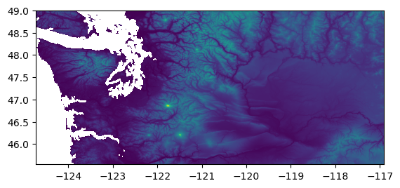
Nice! WA state really does have interesting topography.

• Cascade mountains, Olympic Mountains, Active stratovolcanoes, Puget Sound, Columbia River

• Channeled Scablands: https://en.wikipedia.org/wiki/Channeled_Scablands

Much more interesting than Kansas:

• https://www.usu.edu/geo/geomorph/kansas.html

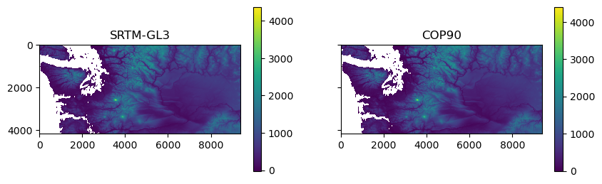
Compare SRTM And Copernicus DEM

Read the data and plot with matplotlib

• Read the data to a NumPy array

  • Note that the tiles on disk are not actually loaded until you read the dataset

  • Make sure you deal with nodata, either with a NumPy masked array, or setting nodata to np.nan (remember np.nan is a float, your input data type is int16)

• View with matplotlib imshow - verify you have a DEM of washington state

srtm_fn = 'WA_SRTMGL3.tif'
cop_fn = 'WA_COP90.tif'

f, axa = plt.subplots(1,2, sharex=True, sharey=True, figsize=(10,3))
#One call to open, read and plot with imshow. Stores output from imshow (mappapble object) to create colorbar
m = axa[0].imshow(rio.open(srtm_fn).read(1, masked=True))
axa[0].set_title('SRTM-GL3')
f.colorbar(m, ax=axa[0])
m = axa[1].imshow(rio.open(cop_fn).read(1, masked=True))
axa[1].set_title('COP90')
f.colorbar(m, ax=axa[1]);

Set nodata value for Copernicus DEM to 0

• Note: The Copernicus DEM creators filled water with values of 0.0 above the EGM2008 geoid (approximates mean sea level)

• We can set these to nodata to conly consider land. This is a bit of a hack, and it is possible that there are real elevations at 0 m that will be masked here.

#Temporarily open file in read/write mode to set nodata value
#https://rasterio.readthedocs.io/en/latest/api/rasterio.html?highlight=open#rasterio.open
with rio.open(cop_fn, 'r+') as src:
    src.nodata = 0.0

Raster reprojection using GDAL and rasterio

Reproject the SRTM DEM to UTM 10N

• The SRTM grids are distributed with crs of EPSG:4326

• Let’s reproject to a more appropriate coordinate system for WA state

  • Use EPSG:32610

dst_crs = 'EPSG:32610'

#Sadly, there is no `to_crs` method as in GeoPandas
#src.to_crs(dst_crs)

First, reproject using gdalwarp command-line utility

• A very simple, efficient way to accomplish this - let GDAL worry about all of the underlying math

• Review the documentation and options here: https://gdal.org/programs/gdalwarp.html

  • Resampling options: https://gdal.org/programs/gdalwarp.html#cmdoption-gdalwarp-r

• Save the projected file as a GeoTiff on disk

  • Use cubic resampling algorithm

• Note the filesize using ls -lh

proj_fn = os.path.splitext(out_fn)[0]+'_utm_gdalwarp.tif'

%%time
if not os.path.exists(proj_fn):
    !gdalwarp -overwrite -r cubic -t_srs $dst_crs $out_fn $proj_fn

CPU times: user 0 ns, sys: 48 µs, total: 48 µs
Wall time: 52.7 µs

ls -lh $proj_fn

-rw-rw-r-- 1 jovyan users 199M Feb 17 01:06 WA_COP90_utm_gdalwarp.tif

!gdalinfo $proj_fn

Driver: GTiff/GeoTIFF
Files: WA_COP90_utm_gdalwarp.tif
Size is 8877, 5851
Coordinate System is:
PROJCRS["WGS 84 / UTM zone 10N",
    BASEGEOGCRS["WGS 84",
        DATUM["World Geodetic System 1984",
            ELLIPSOID["WGS 84",6378137,298.257223563,
                LENGTHUNIT["metre",1]]],
        PRIMEM["Greenwich",0,
            ANGLEUNIT["degree",0.0174532925199433]],
        ID["EPSG",4326]],
    CONVERSION["UTM zone 10N",
        METHOD["Transverse Mercator",
            ID["EPSG",9807]],
        PARAMETER["Latitude of natural origin",0,
            ANGLEUNIT["degree",0.0174532925199433],
            ID["EPSG",8801]],
        PARAMETER["Longitude of natural origin",-123,
            ANGLEUNIT["degree",0.0174532925199433],
            ID["EPSG",8802]],
        PARAMETER["Scale factor at natural origin",0.9996,
            SCALEUNIT["unity",1],
            ID["EPSG",8805]],
        PARAMETER["False easting",500000,
            LENGTHUNIT["metre",1],
            ID["EPSG",8806]],
        PARAMETER["False northing",0,
            LENGTHUNIT["metre",1],
            ID["EPSG",8807]]],
    CS[Cartesian,2],
        AXIS["(E)",east,
            ORDER[1],
            LENGTHUNIT["metre",1]],
        AXIS["(N)",north,
            ORDER[2],
            LENGTHUNIT["metre",1]],
    USAGE[
        SCOPE["Engineering survey, topographic mapping."],
        AREA["Between 126°W and 120°W, northern hemisphere between equator and 84°N, onshore and offshore. Canada - British Columbia (BC); Northwest Territories (NWT); Nunavut; Yukon. United States (USA) - Alaska (AK)."],
        BBOX[0,-126,84,-120]],
    ID["EPSG",32610]]
Data axis to CRS axis mapping: 1,2
Origin = (364685.490899736876599,5445638.415841511450708)
Pixel Size = (68.748471281554814,-68.748471281554814)
Metadata:
  AREA_OR_POINT=Area
Image Structure Metadata:
  INTERLEAVE=BAND
Corner Coordinates:
Upper Left  (  364685.491, 5445638.416) (124d51'20.11"W, 49d 8'55.14"N)
Lower Left  (  364685.491, 5043391.110) (124d43'58.58"W, 45d31'51.28"N)
Upper Right (  974965.670, 5445638.416) (116d30'24.81"W, 48d58'49.93"N)
Lower Right (  974965.670, 5043391.110) (116d55'58.87"W, 45d22'57.49"N)
Center      (  669825.581, 5244514.763) (120d45' 7.90"W, 47d19'55.38"N)
Band 1 Block=8877x1 Type=Float32, ColorInterp=Gray
  NoData Value=0

A note about “creation options” when writing a new file to disk

• Review this great reference on GeoTiff file format: https://www.gdal.org/frmt_gtiff.html

  • See Creation Options section toward bottom of page: https://gdal.org/drivers/raster/gtiff.html#creation-options

• I almost always use -co COMPRESS=LZW -co TILED=YES -co BIGTIFF=IF_SAFER

  • Uses lossless LZW compression (we explored in LS8 example comparing filesize on disk to your calculated array filesize)

  • Writes the tif image in “tiles” of 256x256 px instead of one large block - makes it much more efficient to read and extract a subwindow from the tif

  • If necessary, use the BIGTIFF format for files that are >4 GB

Write out the same file, but this time use tiling and LZW compression

• Compare the new filesize on disk

proj_fn_lzw = os.path.splitext(out_fn)[0]+'_utm_gdalwarp_lzw.tif'

%%time
if not os.path.exists(proj_fn_lzw):
    !gdalwarp -r cubic -t_srs $dst_crs -co COMPRESS=LZW -co TILED=YES -co BIGTIFF=IF_SAFER $out_fn $proj_fn_lzw

CPU times: user 869 µs, sys: 0 ns, total: 869 µs
Wall time: 944 µs

ls -lh $proj_fn_lzw

-rw-rw-r-- 1 jovyan users 176M Feb 17 01:07 WA_COP90_utm_gdalwarp_lzw.tif

#Let's use the compressed file from here on out
#Should compare runtimes when using compressed vs. uncompressed
proj_fn = proj_fn_lzw

!gdalinfo $proj_fn

Driver: GTiff/GeoTIFF
Files: WA_COP90_utm_gdalwarp_lzw.tif
Size is 8877, 5851
Coordinate System is:
PROJCRS["WGS 84 / UTM zone 10N",
    BASEGEOGCRS["WGS 84",
        DATUM["World Geodetic System 1984",
            ELLIPSOID["WGS 84",6378137,298.257223563,
                LENGTHUNIT["metre",1]]],
        PRIMEM["Greenwich",0,
            ANGLEUNIT["degree",0.0174532925199433]],
        ID["EPSG",4326]],
    CONVERSION["UTM zone 10N",
        METHOD["Transverse Mercator",
            ID["EPSG",9807]],
        PARAMETER["Latitude of natural origin",0,
            ANGLEUNIT["degree",0.0174532925199433],
            ID["EPSG",8801]],
        PARAMETER["Longitude of natural origin",-123,
            ANGLEUNIT["degree",0.0174532925199433],
            ID["EPSG",8802]],
        PARAMETER["Scale factor at natural origin",0.9996,
            SCALEUNIT["unity",1],
            ID["EPSG",8805]],
        PARAMETER["False easting",500000,
            LENGTHUNIT["metre",1],
            ID["EPSG",8806]],
        PARAMETER["False northing",0,
            LENGTHUNIT["metre",1],
            ID["EPSG",8807]]],
    CS[Cartesian,2],
        AXIS["(E)",east,
            ORDER[1],
            LENGTHUNIT["metre",1]],
        AXIS["(N)",north,
            ORDER[2],
            LENGTHUNIT["metre",1]],
    USAGE[
        SCOPE["Engineering survey, topographic mapping."],
        AREA["Between 126°W and 120°W, northern hemisphere between equator and 84°N, onshore and offshore. Canada - British Columbia (BC); Northwest Territories (NWT); Nunavut; Yukon. United States (USA) - Alaska (AK)."],
        BBOX[0,-126,84,-120]],
    ID["EPSG",32610]]
Data axis to CRS axis mapping: 1,2
Origin = (364685.490899736876599,5445638.415841511450708)
Pixel Size = (68.748471281554814,-68.748471281554814)
Metadata:
  AREA_OR_POINT=Area
Image Structure Metadata:
  COMPRESSION=LZW
  INTERLEAVE=BAND
Corner Coordinates:
Upper Left  (  364685.491, 5445638.416) (124d51'20.11"W, 49d 8'55.14"N)
Lower Left  (  364685.491, 5043391.110) (124d43'58.58"W, 45d31'51.28"N)
Upper Right (  974965.670, 5445638.416) (116d30'24.81"W, 48d58'49.93"N)
Lower Right (  974965.670, 5043391.110) (116d55'58.87"W, 45d22'57.49"N)
Center      (  669825.581, 5244514.763) (120d45' 7.90"W, 47d19'55.38"N)
Band 1 Block=256x256 Type=Float32, ColorInterp=Gray
  NoData Value=0

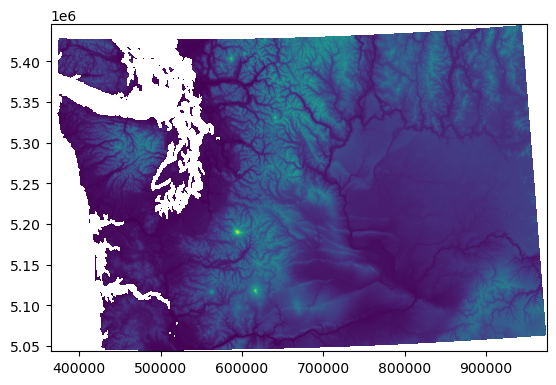
Load your reprojected dataset and plot

with rio.open(proj_fn) as src_proj:
    rio.plot.show(src_proj)

Reprojection using rasterio API

• This is still surprisingly complicated compared to the GeoPandas to_crs method

  • But if you look at what’s actually happening, it’s not too bad

• See example here: https://rasterio.readthedocs.io/en/stable/topics/reproject.html#reprojecting-a-geotiff-dataset

• Define your coordinate system as dst_crs variable (needed later)

• Save the projected file as a GeoTiff on disk

  • print the metadata of your input and output datasets

  • If you are copying the metadata from your input dataset (as in the rasterio doc example), you will need to update the ‘driver’ to ‘GTiff’ before open the file for writing

  • Use cubic resampling algorithm

• You can specify these configuration options in the rasterio.open() kwargs:

  • https://github.com/mapbox/rasterio/blob/master/docs/topics/image_options.rst

  • https://rasterio.readthedocs.io/en/stable/topics/profiles.html

  • https://rasterio.readthedocs.io/en/stable/topics/configuration.html

• Note that it is also possible to reproject and store the resulting dataset in memory, rather than writing to disk

  • This is desirable if you need to temporarily reproject a raster dataset, read the array, do some analysis

def rio_reproj_write(src, proj_fn, dst_crs, driver='GTiff'):
    #Check to see if output filename already exists
    if os.path.exists(proj_fn):
        print("File exists: ", proj_fn)
    else:
        #Get the required transformation and output width and height
        transform, width, height = calculate_default_transform(src.crs, dst_crs, src.width, src.height, *src.bounds)
        #Create a copy of input metadata, then update with output values
        kwargs = src.meta.copy()
        print("Source metadata:\n", kwargs)
        kwargs.update({'crs':dst_crs,'transform':transform,'width':width,'height':height})
        kwargs['driver'] = driver
        #Set output creation options
        kwargs['compress'] = 'LZW'
        kwargs['tiled'] = True
        kwargs['BIGTIFF'] = 'IF_SAFER'
        print("Destination metadata:\n", kwargs)

        #Open the destination dataset in write mode
        with rio.open(proj_fn, 'w', **kwargs) as dst:
            print("Writing: ", proj_fn)
            #Loop through each input band
            for i in range(1, src.count + 1):
                #Reproject!
                reproject(source=rio.band(src, i), destination=rio.band(dst, i), src_transform=src.transform,\
                          src_crs=src.crs, dst_transform=transform, dst_crs=dst_crs, resampling=Resampling.cubic)
            print("Complete")

proj_fn = os.path.splitext(out_fn)[0]+'_utm_riowarp.tif'

with rio.open(out_fn) as src:
    rio_reproj_write(src, proj_fn, dst_crs)

File exists:  WA_COP90_utm_riowarp.tif

src_proj = rio.open(proj_fn)

src_proj.profile

{'driver': 'GTiff', 'dtype': 'float32', 'nodata': 0.0, 'width': 8877, 'height': 5851, 'count': 1, 'crs': CRS.from_epsg(32610), 'transform': Affine(68.74847128155481, 0.0, 364685.4908997369,
       0.0, -68.74847128155481, 5445638.415841511), 'blockxsize': 256, 'blockysize': 256, 'tiled': True, 'compress': 'lzw', 'interleave': 'band'}

src_proj.res

(68.74847128155481, 68.74847128155481)

#Load as a masked array
#dem_proj = src_proj.read(1, masked=True)
#dem_proj.shape

Discussion Questions

• What is the original x and y pixel size and units?

  • Remember this is a 3-arcsecond grid

  • Info on an arcsecond: https://www.esri.com/news/arcuser/0400/wdside.html

• What is the projected x and y pixel size and units?

  • Is this consistent with your expectation for the 90-m Copernicus DEM or 3-arcsec SRTM data?

    • Hint: Think about the dimensions of a pixel in meters near the top and bottom of the unprojected raster.

      • Roughly 45.5° and 49°

    • Then think back to Lab04 when we calculated length of a degree of longitude and a degree of latitude at different locations on the planet. (https://uwgda-jupyterbook.readthedocs.io/en/latest/modules/04_Vector1_Geopandas_CRS_Proj/04_Vector1_Geopandas_CRS_Proj_exercises.html#questions)

src.bounds

BoundingBox(left=-124.73333333333332, bottom=45.543749999999996, right=-116.91583333333332, top=49.002916666666664)

src.res

(0.0008333333333333334, 0.0008333333333333334)

#Approximate length of a degree of latitude
mpd = 111000

src.res[0] * mpd

92.5

src.res[0] * mpd*np.cos(np.radians(src.bounds.top))

60.68190636208666

src.res[0] * mpd*np.cos(np.radians(src.bounds.bottom))

64.78371025007438

src_proj.res

(68.74847128155481, 68.74847128155481)

• Note that if the output resolution is unspecified, GDAL and rasterio will calcluate for you.

  • More info on the default “Suggested Warp Output” resolution: https://gdal.org/api/gdal_alg.html#_CPPv423GDALSuggestedWarpOutput12GDALDatasetH19GDALTransformerFuncPvPdPiPi

…resolution is computed with the intent that the length of the distance from the top left corner of the output imagery to the bottom right corner would represent the same number of pixels as in the source image. Note that if the image is somewhat rotated the diagonal taken isn’t of the whole output bounding rectangle, but instead of the locations where the top/left and bottom/right corners transform. The output pixel size is always square. This is intended to approximately preserve the resolution of the input data in the output file.

• But you can also specify this output resolution (-tr argument in gdalwarp), if, for example, you wanted to resample your output to 180 m resolution.

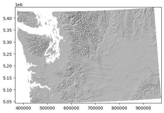
Part 2: Create a shaded relief map (hillshade) from your projected DEM

• See background info on hillshades (and other DEM derivative products like slope and aspect) here: http://desktop.arcgis.com/en/arcmap/10.3/tools/spatial-analyst-toolbox/how-hillshade-works.htm

• Can do this easily with gdaldem command line utility: https://gdal.org/programs/gdaldem.html

  • Try this and output to a new file

  • Note that if you were to run on a DEM with different horizontal and vertical units, (like say, degrees and meters), you will have scaling issues. There are ways around this, but Always generate hillshade using a projected DEM.

hs_fn = os.path.splitext(proj_fn)[0]+'_hs.tif'

%%time
if not os.path.exists(hs_fn):
    !gdaldem hillshade $proj_fn $hs_fn

CPU times: user 25 µs, sys: 9 µs, total: 34 µs
Wall time: 38.6 µs

Use rasterio to load your GDAL shaded relief map as a NumPy masked array

• Note that the datatype is 8-bit (Byte), with values from 0-255 (it’s a grayscale image, not elevation data)

• Make sure you mask nodata values

hs_src = rio.open(hs_fn)
hs = hs_src.read(1, masked=True)

hs_src.profile

{'driver': 'GTiff', 'dtype': 'uint8', 'nodata': 0.0, 'width': 8877, 'height': 5851, 'count': 1, 'crs': CRS.from_epsg(32610), 'transform': Affine(68.74847128155481, 0.0, 364685.4908997369,
       0.0, -68.74847128155481, 5445638.415841511), 'blockysize': 1, 'tiled': False, 'interleave': 'band'}

Get the extent of the hillshade dataset in the projected coordinate system

• See rio.plot.plotting_extent

• Pass this to imshow extent and verify that your coordinates look good

hs_extent = rio.plot.plotting_extent(hs_src)
hs_extent

(364685.4908997369, 974965.6704660989, 5043391.110373134, 5445638.415841511)

f, ax = plt.subplots()
ax.imshow(hs, cmap='gray', extent=hs_extent);

Example of hillshade using GDAL API

• Can also use GDAL Python API directly, rather than command line interface

  • Documentation of this functionality is poor, but it’s pretty simple (see my example below)

  • Some examples are here: https://github.com/OSGeo/gdal/blob/master/autotest/utilities/test_gdaldem_lib.py

def gdal_hs_ds(fn):
    from osgeo import gdal
    #Open the GDAL dataset
    dem_ds = gdal.Open(fn)
    #Specify the type of product we want (e.g., hillshade, slope, aspect) - see gdaldem doc for list of avaiable options
    producttype = 'hillshade'
    #Create a GDAL hillshade dataset in memory
    hs_ds = gdal.DEMProcessing('', dem_ds, 'hillshade', format='MEM')
    return hs_ds

def gdal_hs_ma(fn):
    #Get GDAL Dataset
    hs_ds = gdal_hs_ds(fn)
    #Read the dataset as a NumPy array
    hs = hs_ds.ReadAsArray()
    return hs

#Create hillshade from a filename
#hs_ma = gdal_hs_ma(fn)
#plt.imshow(hs_ma, cmap='gray')

Work in progress: dynamically create shaded relief, slope and aspect using numpy

#Function to return hillshade (for visualization), slope magnitude (deg) and aspect on the fly
#This is a work in progress, aspect values are incorrect!
def hillshade(a, res=1.0, sun_az=315, sun_el=45):
    sun_az = 360.0 - sun_az
    dx, dy = np.gradient(a, res)
    slope = np.pi/2. - np.arctan(np.sqrt(dx*dx + dy*dy))
    aspect = np.arctan2(-dx, dy)
    shaded = np.sin(np.radians(sun_az)) * np.sin(slope) + \
    np.cos(np.radians(sun_el)) * np.cos(slope) * \
    np.cos((np.radians(sun_az) - np.pi/2.) - aspect)
    hs = 255 * (shaded + 1)/2
    return hs, np.degrees(np.pi/2. - slope), np.degrees(aspect)

Part 3: Clipping Raster data

Load the states GeoDataFrame

#states_url = 'http://eric.clst.org/assets/wiki/uploads/Stuff/gz_2010_us_040_00_5m.json'
states_url = 'http://eric.clst.org/assets/wiki/uploads/Stuff/gz_2010_us_040_00_500k.json'
states_gdf = gpd.read_file(states_url)
states_gdf.head()

	GEO_ID	STATE	NAME	LSAD	CENSUSAREA	geometry
0	0400000US23	23	Maine		30842.923	MULTIPOLYGON (((-67.61976 44.51975, -67.61541 ...
1	0400000US25	25	Massachusetts		7800.058	MULTIPOLYGON (((-70.83204 41.60650, -70.82373 ...
2	0400000US26	26	Michigan		56538.901	MULTIPOLYGON (((-88.68443 48.11579, -88.67563 ...
3	0400000US30	30	Montana		145545.801	POLYGON ((-104.05770 44.99743, -104.25015 44.9...
4	0400000US32	32	Nevada		109781.180	POLYGON ((-114.05060 37.00040, -114.04999 36.9...

Reproject the GeoDataFrame to match your DEM

states_gdf_proj = states_gdf.to_crs(dst_crs)

Isolate the WA state geometry object

• We want the geometry, not a GeoDataFrame or GeoSeries

wa_state = states_gdf_proj.loc[states_gdf_proj['NAME'] == 'Washington']
wa_geom = wa_state.iloc[0].geometry

wa_geom

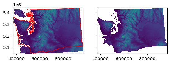
Clip your projected DEM dataset (not the hillshade) to the WA state multipolygon

• This is a common GIS operation

• Some useful resources:

  • https://rasterio.readthedocs.io/en/stable/topics/masking-by-shapefile.html

  • https://automating-gis-processes.github.io/CSC18/lessons/L6/clipping-raster.html

  • https://www.earthdatascience.org/courses/earth-analytics-python/lidar-raster-data/crop-raster-data-with-shapefile-in-python/

• Note that input for rasterio mask is a rasterio dataset, not a numpy array

• Can experiment with different options (which are a bit different than other rasterio syntax):

  • These will return a masked array (and transform) ready for analysis: filled=False, crop=True, indexes=1

• Plot with imshow to verify - you should see a DEM clipped to WA state outline!

  • Use rio.plot.plotting_extent to get the projected coordinate extent, and pass this to the imshow extent

    • https://rasterio.readthedocs.io/en/latest/api/rasterio.plot.html#rasterio.plot.plotting_extent

src_proj

<open DatasetReader name='WA_COP90_utm_riowarp.tif' mode='r'>

#rio.mask.mask?

rio_mask_kwargs = {'filled':False, 'crop':True, 'indexes':1}

rio.mask.mask(src_proj, wa_geom.geoms, **rio_mask_kwargs)

(masked_array(
   data=[[--, --, --, ..., --, --, --],
         [--, --, --, ..., --, --, --],
         [--, --, --, ..., --, --, --],
         ...,
         [--, --, --, ..., --, --, --],
         [--, --, --, ..., --, --, --],
         [--, --, --, ..., --, --, --]],
   mask=[[ True,  True,  True, ...,  True,  True,  True],
         [ True,  True,  True, ...,  True,  True,  True],
         [ True,  True,  True, ...,  True,  True,  True],
         ...,
         [ True,  True,  True, ...,  True,  True,  True],
         [ True,  True,  True, ...,  True,  True,  True],
         [ True,  True,  True, ...,  True,  True,  True]],
   fill_value=0.0,
   dtype=float32),
 Affine(68.74847128155481, 0.0, 371079.0987289215,
        0.0, -68.74847128155481, 5444607.188772288))

src_proj.transform

Affine(68.74847128155481, 0.0, 364685.4908997369,
       0.0, -68.74847128155481, 5445638.415841511)

#No need to do read here, masked array directly loaded from disk
wa_ma, wa_ma_transform = rio.mask.mask(src_proj, wa_geom.geoms, **rio_mask_kwargs)

wa_ma.shape

(5834, 8728)

wa_ma_transform

Affine(68.74847128155481, 0.0, 371079.0987289215,
       0.0, -68.74847128155481, 5444607.188772288)

#Get clipped extent in UTM coordaintes
wa_ma_extent = rio.plot.plotting_extent(wa_ma, wa_ma_transform)
wa_ma_extent

(371079.0987289215, 971115.7560743319, 5043528.607315698, 5444607.188772288)

#Original unclipped extent for comparison
src_proj.bounds

BoundingBox(left=364685.4908997369, bottom=5043391.110373134, right=974965.6704660989, top=5445638.415841511)

f, axa = plt.subplots(1, 2, sharex=True, sharey=True)
axa[0].imshow(src_proj.read(1, masked=True), extent=wa_ma_extent)
wa_state.plot(ax=axa[0], facecolor='none', edgecolor='r')
axa[1].imshow(wa_ma, extent=wa_ma_extent);

Part 4: Comparing and differencing rasters

• Often have two rasters with different resolution, extent, projection

• Want to combine, or use for some kind of raster math (e.g., subtract one from the other to compute difference)

• Relatively new package, rioxarray makes this very easy

  • https://corteva.github.io/rioxarray/stable/index.html

  • More on this in Week09 and Week10

  • Built for NetCDF model, but wraps rasterio for working with rasters

  • Lazy evaluation, doesn’t read from disk util necessary

  • Built-in support for parallel operations using Dask

#Original SRTM DEM, still in EPSG:4326
srtm_fn

'WA_SRTMGL3.tif'

#Projected COP DEM, reprojected in EPSG:32610
proj_fn

'WA_COP90_utm_riowarp.tif'

Open using rioxarray

• Open the two GeoTiff products as xarray DataSets (more on this in Week09)

  • https://corteva.github.io/rioxarray/html/rioxarray.html#rioxarray-open-rasterio

• Check out the spatial_ref attribute and access CRS

  • https://corteva.github.io/rioxarray/stable/getting_started/crs_management.html

rioxarray.open_rasterio(proj_fn, masked=True)

<xarray.DataArray (band: 1, y: 5851, x: 8877)>
[51939327 values with dtype=float32]
Coordinates:
  * band         (band) int64 1
  * x            (x) float64 3.647e+05 3.648e+05 ... 9.749e+05 9.749e+05
  * y            (y) float64 5.446e+06 5.446e+06 ... 5.043e+06 5.043e+06
    spatial_ref  int64 0
Attributes:
    AREA_OR_POINT:  Area
    scale_factor:   1.0
    add_offset:     0.0

xarray.DataArray

• band: 1
• y: 5851
• x: 8877

• ...

  [51939327 values with dtype=float32]

• Coordinates: (4)
  • band
    (band)
    int64
    1

    array([1])

  • x
    (x)
    float64
    3.647e+05 3.648e+05 ... 9.749e+05

    array([364719.865135, 364788.613607, 364857.362078, ..., 974793.799288,
           974862.547759, 974931.29623 ])

  • y
    (y)
    float64
    5.446e+06 5.446e+06 ... 5.043e+06

    array([5445604.041606, 5445535.293135, 5445466.544663, ..., 5043562.981551,
           5043494.23308 , 5043425.484609])

  • spatial_ref
    ()
    int64
    0

    crs_wkt :

    PROJCS["WGS 84 / UTM zone 10N",GEOGCS["WGS 84",DATUM["WGS_1984",SPHEROID["WGS 84",6378137,298.257223563,AUTHORITY["EPSG","7030"]],AUTHORITY["EPSG","6326"]],PRIMEM["Greenwich",0,AUTHORITY["EPSG","8901"]],UNIT["degree",0.0174532925199433,AUTHORITY["EPSG","9122"]],AUTHORITY["EPSG","4326"]],PROJECTION["Transverse_Mercator"],PARAMETER["latitude_of_origin",0],PARAMETER["central_meridian",-123],PARAMETER["scale_factor",0.9996],PARAMETER["false_easting",500000],PARAMETER["false_northing",0],UNIT["metre",1,AUTHORITY["EPSG","9001"]],AXIS["Easting",EAST],AXIS["Northing",NORTH],AUTHORITY["EPSG","32610"]]

    semi_major_axis :

    6378137.0

    semi_minor_axis :

    6356752.314245179

    inverse_flattening :

    298.257223563

    reference_ellipsoid_name :

    WGS 84

    longitude_of_prime_meridian :

    0.0

    prime_meridian_name :

    Greenwich

    geographic_crs_name :

    WGS 84

    horizontal_datum_name :

    World Geodetic System 1984

    projected_crs_name :

    WGS 84 / UTM zone 10N

    grid_mapping_name :

    transverse_mercator

    latitude_of_projection_origin :

    0.0

    longitude_of_central_meridian :

    -123.0

    false_easting :

    500000.0

    false_northing :

    0.0

    scale_factor_at_central_meridian :

    0.9996

    spatial_ref :

    PROJCS["WGS 84 / UTM zone 10N",GEOGCS["WGS 84",DATUM["WGS_1984",SPHEROID["WGS 84",6378137,298.257223563,AUTHORITY["EPSG","7030"]],AUTHORITY["EPSG","6326"]],PRIMEM["Greenwich",0,AUTHORITY["EPSG","8901"]],UNIT["degree",0.0174532925199433,AUTHORITY["EPSG","9122"]],AUTHORITY["EPSG","4326"]],PROJECTION["Transverse_Mercator"],PARAMETER["latitude_of_origin",0],PARAMETER["central_meridian",-123],PARAMETER["scale_factor",0.9996],PARAMETER["false_easting",500000],PARAMETER["false_northing",0],UNIT["metre",1,AUTHORITY["EPSG","9001"]],AXIS["Easting",EAST],AXIS["Northing",NORTH],AUTHORITY["EPSG","32610"]]

    GeoTransform :

    364685.4908997369 68.74847128155481 0.0 5445638.415841511 0.0 -68.74847128155481

    array(0)

• Indexes: (3)
  • band
    PandasIndex

    PandasIndex(Int64Index([1], dtype='int64', name='band'))

  • x
    PandasIndex

    PandasIndex(Float64Index([ 364719.8651353777, 364788.61360665923,  364857.3620779408,
                   364926.1105492223,  364994.8590205039,  365063.6074917854,
                  365132.35596306704,  365201.1044343486, 365269.85290563013,
                   365338.6013769117,
                  ...
                   974312.5599889243,  974381.3084602058,  974450.0569314873,
                   974518.8054027688,  974587.5538740505,   974656.302345332,
                   974725.0508166135,  974793.7992878952,  974862.5477591767,
                   974931.2962304582],
                 dtype='float64', name='x', length=8877))

  • y
    PandasIndex

    PandasIndex(Float64Index([  5445604.04160587,  5445535.293134589,  5445466.544663307,
                   5445397.796192026,  5445329.047720744,  5445260.299249463,
                   5445191.550778181,    5445122.8023069,  5445054.053835617,
                   5444985.305364336,
                  ...
                   5044044.220850308,  5043975.472379027,  5043906.723907745,
                   5043837.975436464,  5043769.226965182,  5043700.478493901,
                  5043631.7300226195,  5043562.981551338, 5043494.2330800565,
                   5043425.484608775],
                 dtype='float64', name='y', length=5851))

• Attributes: (3)

  AREA_OR_POINT :

  Area

  scale_factor :

  1.0

  add_offset :

  0.0

#Note: since nodata is set, we can use masked=True to set those values to nan
#Using squeeze here to reduce the band=1 dimension
cop_xds = rioxarray.open_rasterio(proj_fn, masked=True).squeeze()
cop_xds

<xarray.DataArray (y: 5851, x: 8877)>
[51939327 values with dtype=float32]
Coordinates:
    band         int64 1
  * x            (x) float64 3.647e+05 3.648e+05 ... 9.749e+05 9.749e+05
  * y            (y) float64 5.446e+06 5.446e+06 ... 5.043e+06 5.043e+06
    spatial_ref  int64 0
Attributes:
    AREA_OR_POINT:  Area
    scale_factor:   1.0
    add_offset:     0.0

xarray.DataArray

• y: 5851
• x: 8877

• ...

  [51939327 values with dtype=float32]

• Coordinates: (4)
  • band
    ()
    int64
    1

    array(1)

  • x
    (x)
    float64
    3.647e+05 3.648e+05 ... 9.749e+05

    array([364719.865135, 364788.613607, 364857.362078, ..., 974793.799288,
           974862.547759, 974931.29623 ])

  • y
    (y)
    float64
    5.446e+06 5.446e+06 ... 5.043e+06

    array([5445604.041606, 5445535.293135, 5445466.544663, ..., 5043562.981551,
           5043494.23308 , 5043425.484609])

  • spatial_ref
    ()
    int64
    0

    crs_wkt :

    PROJCS["WGS 84 / UTM zone 10N",GEOGCS["WGS 84",DATUM["WGS_1984",SPHEROID["WGS 84",6378137,298.257223563,AUTHORITY["EPSG","7030"]],AUTHORITY["EPSG","6326"]],PRIMEM["Greenwich",0,AUTHORITY["EPSG","8901"]],UNIT["degree",0.0174532925199433,AUTHORITY["EPSG","9122"]],AUTHORITY["EPSG","4326"]],PROJECTION["Transverse_Mercator"],PARAMETER["latitude_of_origin",0],PARAMETER["central_meridian",-123],PARAMETER["scale_factor",0.9996],PARAMETER["false_easting",500000],PARAMETER["false_northing",0],UNIT["metre",1,AUTHORITY["EPSG","9001"]],AXIS["Easting",EAST],AXIS["Northing",NORTH],AUTHORITY["EPSG","32610"]]

    semi_major_axis :

    6378137.0

    semi_minor_axis :

    6356752.314245179

    inverse_flattening :

    298.257223563

    reference_ellipsoid_name :

    WGS 84

    longitude_of_prime_meridian :

    0.0

    prime_meridian_name :

    Greenwich

    geographic_crs_name :

    WGS 84

    horizontal_datum_name :

    World Geodetic System 1984

    projected_crs_name :

    WGS 84 / UTM zone 10N

    grid_mapping_name :

    transverse_mercator

    latitude_of_projection_origin :

    0.0

    longitude_of_central_meridian :

    -123.0

    false_easting :

    500000.0

    false_northing :

    0.0

    scale_factor_at_central_meridian :

    0.9996

    spatial_ref :

    PROJCS["WGS 84 / UTM zone 10N",GEOGCS["WGS 84",DATUM["WGS_1984",SPHEROID["WGS 84",6378137,298.257223563,AUTHORITY["EPSG","7030"]],AUTHORITY["EPSG","6326"]],PRIMEM["Greenwich",0,AUTHORITY["EPSG","8901"]],UNIT["degree",0.0174532925199433,AUTHORITY["EPSG","9122"]],AUTHORITY["EPSG","4326"]],PROJECTION["Transverse_Mercator"],PARAMETER["latitude_of_origin",0],PARAMETER["central_meridian",-123],PARAMETER["scale_factor",0.9996],PARAMETER["false_easting",500000],PARAMETER["false_northing",0],UNIT["metre",1,AUTHORITY["EPSG","9001"]],AXIS["Easting",EAST],AXIS["Northing",NORTH],AUTHORITY["EPSG","32610"]]

    GeoTransform :

    364685.4908997369 68.74847128155481 0.0 5445638.415841511 0.0 -68.74847128155481

    array(0)

• Indexes: (2)
  • x
    PandasIndex

    PandasIndex(Float64Index([ 364719.8651353777, 364788.61360665923,  364857.3620779408,
                   364926.1105492223,  364994.8590205039,  365063.6074917854,
                  365132.35596306704,  365201.1044343486, 365269.85290563013,
                   365338.6013769117,
                  ...
                   974312.5599889243,  974381.3084602058,  974450.0569314873,
                   974518.8054027688,  974587.5538740505,   974656.302345332,
                   974725.0508166135,  974793.7992878952,  974862.5477591767,
                   974931.2962304582],
                 dtype='float64', name='x', length=8877))

  • y
    PandasIndex

    PandasIndex(Float64Index([  5445604.04160587,  5445535.293134589,  5445466.544663307,
                   5445397.796192026,  5445329.047720744,  5445260.299249463,
                   5445191.550778181,    5445122.8023069,  5445054.053835617,
                   5444985.305364336,
                  ...
                   5044044.220850308,  5043975.472379027,  5043906.723907745,
                   5043837.975436464,  5043769.226965182,  5043700.478493901,
                  5043631.7300226195,  5043562.981551338, 5043494.2330800565,
                   5043425.484608775],
                 dtype='float64', name='y', length=5851))

• Attributes: (3)

  AREA_OR_POINT :

  Area

  scale_factor :

  1.0

  add_offset :

  0.0

Access rasterio functions/attributes

#cop_xds.rio.

cop_xds.rio.crs

CRS.from_epsg(32610)

Quick plotting using xarray

• https://xarray.pydata.org/en/stable/generated/xarray.plot.imshow.html

#Default xarray plot uses the contourf method - can fill memory!
#cop_xds.plot()

xarray use RdBu and symmetrical color bar here when negative values detected

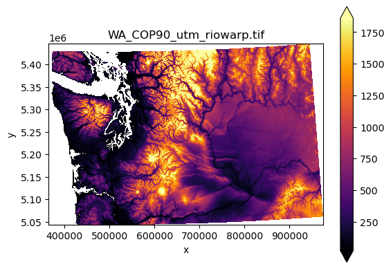
cop_xds.plot.imshow();

f, ax = plt.subplots()
cop_xds.plot.imshow(cmap='inferno', robust=True, ax=ax)
ax.set_aspect('equal')
ax.set_title(proj_fn);

Clipping with rioxarray

• https://corteva.github.io/rioxarray/stable/examples/clip_geom.html

#One liner
cop_xds_wa = cop_xds.rio.clip(wa_state.geometry)

f, ax = plt.subplots()
cop_xds_wa.plot.imshow(cmap='inferno', robust=True, ax=ax)
ax.set_aspect('equal')

cop_xds_wa.max()

<xarray.DataArray ()>
array(4399.989, dtype=float32)
Coordinates:
    band         int64 1
    spatial_ref  int64 0

xarray.DataArray

• 4.4e+03

  array(4399.989, dtype=float32)

• Coordinates: (2)
  • band
    ()
    int64
    1

    array(1)

  • spatial_ref
    ()
    int64
    0

    crs_wkt :

    PROJCS["WGS 84 / UTM zone 10N",GEOGCS["WGS 84",DATUM["WGS_1984",SPHEROID["WGS 84",6378137,298.257223563,AUTHORITY["EPSG","7030"]],AUTHORITY["EPSG","6326"]],PRIMEM["Greenwich",0,AUTHORITY["EPSG","8901"]],UNIT["degree",0.0174532925199433,AUTHORITY["EPSG","9122"]],AUTHORITY["EPSG","4326"]],PROJECTION["Transverse_Mercator"],PARAMETER["latitude_of_origin",0],PARAMETER["central_meridian",-123],PARAMETER["scale_factor",0.9996],PARAMETER["false_easting",500000],PARAMETER["false_northing",0],UNIT["metre",1,AUTHORITY["EPSG","9001"]],AXIS["Easting",EAST],AXIS["Northing",NORTH],AUTHORITY["EPSG","32610"]]

    semi_major_axis :

    6378137.0

    semi_minor_axis :

    6356752.314245179

    inverse_flattening :

    298.257223563

    reference_ellipsoid_name :

    WGS 84

    longitude_of_prime_meridian :

    0.0

    prime_meridian_name :

    Greenwich

    geographic_crs_name :

    WGS 84

    horizontal_datum_name :

    World Geodetic System 1984

    projected_crs_name :

    WGS 84 / UTM zone 10N

    grid_mapping_name :

    transverse_mercator

    latitude_of_projection_origin :

    0.0

    longitude_of_central_meridian :

    -123.0

    false_easting :

    500000.0

    false_northing :

    0.0

    scale_factor_at_central_meridian :

    0.9996

    spatial_ref :

    PROJCS["WGS 84 / UTM zone 10N",GEOGCS["WGS 84",DATUM["WGS_1984",SPHEROID["WGS 84",6378137,298.257223563,AUTHORITY["EPSG","7030"]],AUTHORITY["EPSG","6326"]],PRIMEM["Greenwich",0,AUTHORITY["EPSG","8901"]],UNIT["degree",0.0174532925199433,AUTHORITY["EPSG","9122"]],AUTHORITY["EPSG","4326"]],PROJECTION["Transverse_Mercator"],PARAMETER["latitude_of_origin",0],PARAMETER["central_meridian",-123],PARAMETER["scale_factor",0.9996],PARAMETER["false_easting",500000],PARAMETER["false_northing",0],UNIT["metre",1,AUTHORITY["EPSG","9001"]],AXIS["Easting",EAST],AXIS["Northing",NORTH],AUTHORITY["EPSG","32610"]]

    GeoTransform :

    371147.84720020305 68.74847128155483 0.0 5444538.440301007 0.0 -68.74847128155479

    array(0)

• Indexes: (0)
• Attributes: (0)

Open unprojected SRTM file

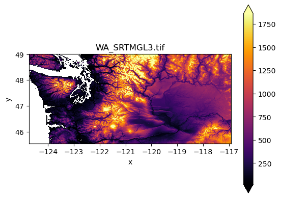
srtm_xds = rioxarray.open_rasterio(srtm_fn, masked=True).squeeze()

srtm_xds

<xarray.DataArray (y: 4151, x: 9381)>
[38940531 values with dtype=float32]
Coordinates:
    band         int64 1
  * x            (x) float64 -124.7 -124.7 -124.7 ... -116.9 -116.9 -116.9
  * y            (y) float64 49.0 49.0 49.0 49.0 ... 45.55 45.55 45.55 45.54
    spatial_ref  int64 0
Attributes:
    AREA_OR_POINT:  Area
    scale_factor:   1.0
    add_offset:     0.0

xarray.DataArray

• y: 4151
• x: 9381

• ...

  [38940531 values with dtype=float32]

• Coordinates: (4)
  • band
    ()
    int64
    1

    array(1)

  • x
    (x)
    float64
    -124.7 -124.7 ... -116.9 -116.9

    array([-124.733333, -124.7325  , -124.731667, ..., -116.918333, -116.9175  ,
           -116.916667])

  • y
    (y)
    float64
    49.0 49.0 49.0 ... 45.55 45.54

    array([49.0025  , 49.001667, 49.000833, ..., 45.545833, 45.545   , 45.544167])

  • spatial_ref
    ()
    int64
    0

    crs_wkt :

    GEOGCS["WGS 84",DATUM["WGS_1984",SPHEROID["WGS 84",6378137,298.257223563,AUTHORITY["EPSG","7030"]],AUTHORITY["EPSG","6326"]],PRIMEM["Greenwich",0,AUTHORITY["EPSG","8901"]],UNIT["degree",0.0174532925199433,AUTHORITY["EPSG","9122"]],AXIS["Latitude",NORTH],AXIS["Longitude",EAST],AUTHORITY["EPSG","4326"]]

    semi_major_axis :

    6378137.0

    semi_minor_axis :

    6356752.314245179

    inverse_flattening :

    298.257223563

    reference_ellipsoid_name :

    WGS 84

    longitude_of_prime_meridian :

    0.0

    prime_meridian_name :

    Greenwich

    geographic_crs_name :

    WGS 84

    grid_mapping_name :

    latitude_longitude

    spatial_ref :

    GEOGCS["WGS 84",DATUM["WGS_1984",SPHEROID["WGS 84",6378137,298.257223563,AUTHORITY["EPSG","7030"]],AUTHORITY["EPSG","6326"]],PRIMEM["Greenwich",0,AUTHORITY["EPSG","8901"]],UNIT["degree",0.0174532925199433,AUTHORITY["EPSG","9122"]],AXIS["Latitude",NORTH],AXIS["Longitude",EAST],AUTHORITY["EPSG","4326"]]

    GeoTransform :

    -124.73375000001255 0.000833333333333144 0.0 49.002916666669165 0.0 -0.000833333333333144

    array(0)

• Indexes: (2)
  • x
    PandasIndex

    PandasIndex(Float64Index([-124.73333333334588, -124.73250000001255, -124.73166666667922,
                  -124.73083333334588, -124.73000000001255, -124.72916666667922,
                  -124.72833333334589, -124.72750000001255, -124.72666666667922,
                  -124.72583333334589,
                  ...
                  -116.92416666668099, -116.92333333334766, -116.92250000001432,
                  -116.92166666668099, -116.92083333334766, -116.92000000001433,
                    -116.919166666681, -116.91833333334766, -116.91750000001433,
                    -116.916666666681],
                 dtype='float64', name='x', length=9381))

  • y
    PandasIndex

    PandasIndex(Float64Index([  49.0025000000025, 49.001666666669166, 49.000833333335834,
                    49.0000000000025,  48.99916666666917, 48.998333333335836,
                    48.9975000000025, 48.996666666669164,  48.99583333333583,
                    48.9950000000025,
                  ...
                   45.55166666666995,  45.55083333333662,  45.55000000000328,
                   45.54916666666995, 45.548333333336615,  45.54750000000328,
                   45.54666666666995,  45.54583333333662, 45.545000000003284,
                   45.54416666666995],
                 dtype='float64', name='y', length=4151))

• Attributes: (3)

  AREA_OR_POINT :

  Area

  scale_factor :

  1.0

  add_offset :

  0.0

srtm_xds.rio.crs

CRS.from_epsg(4326)

f, ax = plt.subplots()
srtm_xds.plot.imshow(cmap='inferno', robust=True, ax=ax)
ax.set_aspect('equal')
ax.set_title(srtm_fn);

srtm_xds.max()

<xarray.DataArray ()>
array(4371., dtype=float32)
Coordinates:
    band         int64 1
    spatial_ref  int64 0

xarray.DataArray

• 4.371e+03

  array(4371., dtype=float32)

• Coordinates: (2)
  • band
    ()
    int64
    1

    array(1)

  • spatial_ref
    ()
    int64
    0

    crs_wkt :

    GEOGCS["WGS 84",DATUM["WGS_1984",SPHEROID["WGS 84",6378137,298.257223563,AUTHORITY["EPSG","7030"]],AUTHORITY["EPSG","6326"]],PRIMEM["Greenwich",0,AUTHORITY["EPSG","8901"]],UNIT["degree",0.0174532925199433,AUTHORITY["EPSG","9122"]],AXIS["Latitude",NORTH],AXIS["Longitude",EAST],AUTHORITY["EPSG","4326"]]

    semi_major_axis :

    6378137.0

    semi_minor_axis :

    6356752.314245179

    inverse_flattening :

    298.257223563

    reference_ellipsoid_name :

    WGS 84

    longitude_of_prime_meridian :

    0.0

    prime_meridian_name :

    Greenwich

    geographic_crs_name :

    WGS 84

    grid_mapping_name :

    latitude_longitude

    spatial_ref :

    GEOGCS["WGS 84",DATUM["WGS_1984",SPHEROID["WGS 84",6378137,298.257223563,AUTHORITY["EPSG","7030"]],AUTHORITY["EPSG","6326"]],PRIMEM["Greenwich",0,AUTHORITY["EPSG","8901"]],UNIT["degree",0.0174532925199433,AUTHORITY["EPSG","9122"]],AXIS["Latitude",NORTH],AXIS["Longitude",EAST],AUTHORITY["EPSG","4326"]]

    GeoTransform :

    -124.73375000001255 0.000833333333333144 0.0 49.002916666669165 0.0 -0.000833333333333144

    array(0)

• Indexes: (0)
• Attributes: (0)

#Try to difference - no output, need to reproject
#cop_xds - srtm_xds

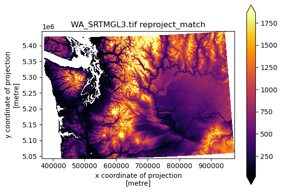
Reproject and match

• Use the rioxarray reproject_match function

  • https://corteva.github.io/rioxarray/stable/examples/reproject_match.html

  • Uses nearest neighbor by default.

    • See available resampling options: https://rasterio.readthedocs.io/en/stable/api/rasterio.enums.html#rasterio.enums.Resampling

#Using cubic resampling (3)
srtm_xds_proj = srtm_xds.rio.reproject_match(cop_xds, resampling=3)

srtm_xds_proj

<xarray.DataArray (y: 5851, x: 8877)>
array([[nan, nan, nan, ..., nan, nan, nan],
       [nan, nan, nan, ..., nan, nan, nan],
       [nan, nan, nan, ..., nan, nan, nan],
       ...,
       [nan, nan, nan, ..., nan, nan, nan],
       [nan, nan, nan, ..., nan, nan, nan],
       [nan, nan, nan, ..., nan, nan, nan]], dtype=float32)
Coordinates:
  * x            (x) float64 3.647e+05 3.648e+05 ... 9.749e+05 9.749e+05
  * y            (y) float64 5.446e+06 5.446e+06 ... 5.043e+06 5.043e+06
    band         int64 1
    spatial_ref  int64 0
Attributes:
    AREA_OR_POINT:  Area
    scale_factor:   1.0
    add_offset:     0.0

xarray.DataArray

• y: 5851
• x: 8877

• nan nan nan nan nan nan nan nan ... nan nan nan nan nan nan nan nan

  array([[nan, nan, nan, ..., nan, nan, nan],
         [nan, nan, nan, ..., nan, nan, nan],
         [nan, nan, nan, ..., nan, nan, nan],
         ...,
         [nan, nan, nan, ..., nan, nan, nan],
         [nan, nan, nan, ..., nan, nan, nan],
         [nan, nan, nan, ..., nan, nan, nan]], dtype=float32)

• Coordinates: (4)
  • x
    (x)
    float64
    3.647e+05 3.648e+05 ... 9.749e+05

    axis :

    X

    long_name :

    x coordinate of projection

    standard_name :

    projection_x_coordinate

    units :

    metre

    array([364719.865135, 364788.613607, 364857.362078, ..., 974793.799288,
           974862.547759, 974931.29623 ])

  • y
    (y)
    float64
    5.446e+06 5.446e+06 ... 5.043e+06

    axis :

    Y

    long_name :

    y coordinate of projection

    standard_name :

    projection_y_coordinate

    units :

    metre

    array([5445604.041606, 5445535.293135, 5445466.544663, ..., 5043562.981551,
           5043494.23308 , 5043425.484609])

  • band
    ()
    int64
    1

    array(1)

  • spatial_ref
    ()
    int64
    0

    crs_wkt :

    PROJCS["WGS 84 / UTM zone 10N",GEOGCS["WGS 84",DATUM["WGS_1984",SPHEROID["WGS 84",6378137,298.257223563,AUTHORITY["EPSG","7030"]],AUTHORITY["EPSG","6326"]],PRIMEM["Greenwich",0,AUTHORITY["EPSG","8901"]],UNIT["degree",0.0174532925199433,AUTHORITY["EPSG","9122"]],AUTHORITY["EPSG","4326"]],PROJECTION["Transverse_Mercator"],PARAMETER["latitude_of_origin",0],PARAMETER["central_meridian",-123],PARAMETER["scale_factor",0.9996],PARAMETER["false_easting",500000],PARAMETER["false_northing",0],UNIT["metre",1,AUTHORITY["EPSG","9001"]],AXIS["Easting",EAST],AXIS["Northing",NORTH],AUTHORITY["EPSG","32610"]]

    semi_major_axis :

    6378137.0

    semi_minor_axis :

    6356752.314245179

    inverse_flattening :

    298.257223563

    reference_ellipsoid_name :

    WGS 84

    longitude_of_prime_meridian :

    0.0

    prime_meridian_name :

    Greenwich

    geographic_crs_name :

    WGS 84

    horizontal_datum_name :

    World Geodetic System 1984

    projected_crs_name :

    WGS 84 / UTM zone 10N

    grid_mapping_name :

    transverse_mercator

    latitude_of_projection_origin :

    0.0

    longitude_of_central_meridian :

    -123.0

    false_easting :

    500000.0

    false_northing :

    0.0

    scale_factor_at_central_meridian :

    0.9996

    spatial_ref :

    PROJCS["WGS 84 / UTM zone 10N",GEOGCS["WGS 84",DATUM["WGS_1984",SPHEROID["WGS 84",6378137,298.257223563,AUTHORITY["EPSG","7030"]],AUTHORITY["EPSG","6326"]],PRIMEM["Greenwich",0,AUTHORITY["EPSG","8901"]],UNIT["degree",0.0174532925199433,AUTHORITY["EPSG","9122"]],AUTHORITY["EPSG","4326"]],PROJECTION["Transverse_Mercator"],PARAMETER["latitude_of_origin",0],PARAMETER["central_meridian",-123],PARAMETER["scale_factor",0.9996],PARAMETER["false_easting",500000],PARAMETER["false_northing",0],UNIT["metre",1,AUTHORITY["EPSG","9001"]],AXIS["Easting",EAST],AXIS["Northing",NORTH],AUTHORITY["EPSG","32610"]]

    GeoTransform :

    364685.4908997369 68.7484712815548 0.0 5445638.415841511 0.0 -68.74847128155474

    array(0)

• Indexes: (2)
  • x
    PandasIndex

    PandasIndex(Float64Index([ 364719.8651353777, 364788.61360665923,  364857.3620779408,
                   364926.1105492223,  364994.8590205039,  365063.6074917854,
                  365132.35596306704,  365201.1044343486, 365269.85290563013,
                   365338.6013769117,
                  ...
                   974312.5599889243,  974381.3084602058,  974450.0569314873,
                   974518.8054027688,  974587.5538740505,   974656.302345332,
                   974725.0508166135,  974793.7992878952,  974862.5477591767,
                   974931.2962304582],
                 dtype='float64', name='x', length=8877))

  • y
    PandasIndex

    PandasIndex(Float64Index([  5445604.04160587,  5445535.293134589,  5445466.544663307,
                   5445397.796192026,  5445329.047720744,  5445260.299249463,
                   5445191.550778181,    5445122.8023069,  5445054.053835617,
                   5444985.305364336,
                  ...
                   5044044.220850308,  5043975.472379027,  5043906.723907745,
                   5043837.975436464,  5043769.226965182,  5043700.478493901,
                  5043631.7300226195,  5043562.981551338, 5043494.2330800565,
                   5043425.484608775],
                 dtype='float64', name='y', length=5851))

• Attributes: (3)

  AREA_OR_POINT :

  Area

  scale_factor :

  1.0

  add_offset :

  0.0

srtm_xds_proj.rio.crs

CRS.from_epsg(32610)

f, ax = plt.subplots()
srtm_xds_proj.plot.imshow(cmap='inferno', robust=True, ax=ax)
ax.set_aspect('equal')
ax.set_title(srtm_fn+' reproject_match');

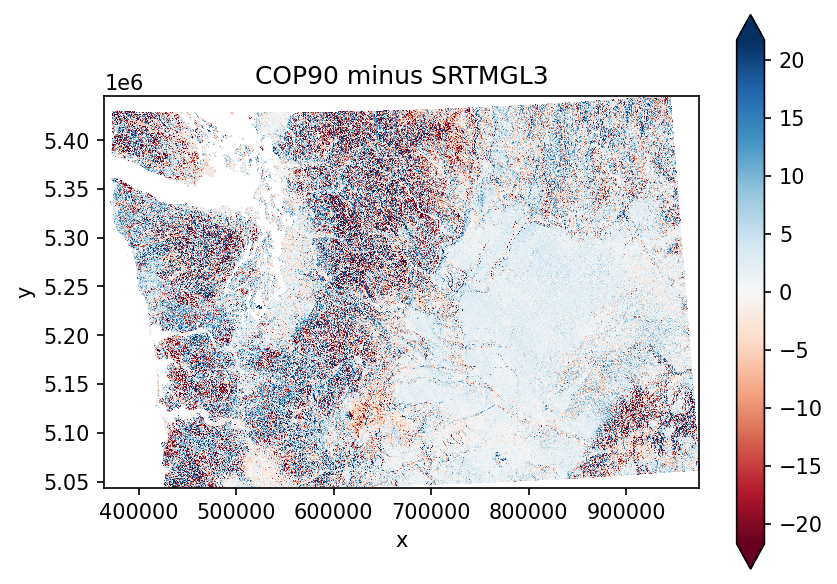
Create a difference map

• Now that both rasters have identical projection, extent, and resolution, this is a simple subtraction

diff = cop_xds - srtm_xds_proj

f, ax = plt.subplots(dpi=150)
diff.plot.imshow(cmap='RdBu', robust=True, ax=ax)
ax.set_aspect('equal')
ax.set_title('COP90 minus SRTMGL3')

Text(0.5, 1.0, 'COP90 minus SRTMGL3')

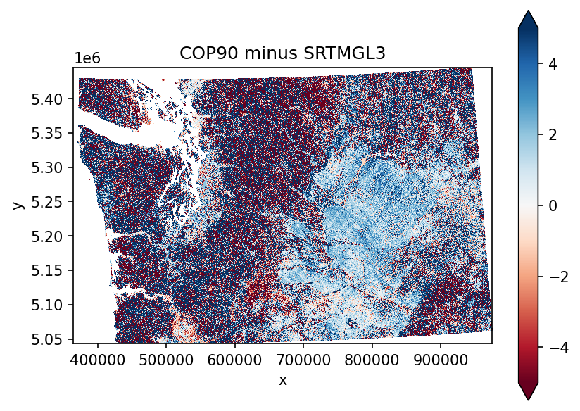
f, ax = plt.subplots(dpi=150)
diff.plot.imshow(cmap='RdBu', robust=True, vmin=-5, vmax=5, ax=ax)
ax.set_aspect('equal')
ax.set_title('COP90 minus SRTMGL3')

Text(0.5, 1.0, 'COP90 minus SRTMGL3')

diff.median()

<xarray.DataArray ()>
array(1.4493103, dtype=float32)
Coordinates:
    band         int64 1
    spatial_ref  int64 0

xarray.DataArray

• 1.449

  array(1.4493103, dtype=float32)

• Coordinates: (2)
  • band
    ()
    int64
    1

    array(1)

  • spatial_ref
    ()
    int64
    0

    crs_wkt :

    PROJCS["WGS 84 / UTM zone 10N",GEOGCS["WGS 84",DATUM["WGS_1984",SPHEROID["WGS 84",6378137,298.257223563,AUTHORITY["EPSG","7030"]],AUTHORITY["EPSG","6326"]],PRIMEM["Greenwich",0,AUTHORITY["EPSG","8901"]],UNIT["degree",0.0174532925199433,AUTHORITY["EPSG","9122"]],AUTHORITY["EPSG","4326"]],PROJECTION["Transverse_Mercator"],PARAMETER["latitude_of_origin",0],PARAMETER["central_meridian",-123],PARAMETER["scale_factor",0.9996],PARAMETER["false_easting",500000],PARAMETER["false_northing",0],UNIT["metre",1,AUTHORITY["EPSG","9001"]],AXIS["Easting",EAST],AXIS["Northing",NORTH],AUTHORITY["EPSG","32610"]]

    semi_major_axis :

    6378137.0

    semi_minor_axis :

    6356752.314245179

    inverse_flattening :

    298.257223563

    reference_ellipsoid_name :

    WGS 84

    longitude_of_prime_meridian :

    0.0

    prime_meridian_name :

    Greenwich

    geographic_crs_name :

    WGS 84

    horizontal_datum_name :

    World Geodetic System 1984

    projected_crs_name :

    WGS 84 / UTM zone 10N

    grid_mapping_name :

    transverse_mercator

    latitude_of_projection_origin :

    0.0

    longitude_of_central_meridian :

    -123.0

    false_easting :

    500000.0

    false_northing :

    0.0

    scale_factor_at_central_meridian :

    0.9996

    spatial_ref :

    PROJCS["WGS 84 / UTM zone 10N",GEOGCS["WGS 84",DATUM["WGS_1984",SPHEROID["WGS 84",6378137,298.257223563,AUTHORITY["EPSG","7030"]],AUTHORITY["EPSG","6326"]],PRIMEM["Greenwich",0,AUTHORITY["EPSG","8901"]],UNIT["degree",0.0174532925199433,AUTHORITY["EPSG","9122"]],AUTHORITY["EPSG","4326"]],PROJECTION["Transverse_Mercator"],PARAMETER["latitude_of_origin",0],PARAMETER["central_meridian",-123],PARAMETER["scale_factor",0.9996],PARAMETER["false_easting",500000],PARAMETER["false_northing",0],UNIT["metre",1,AUTHORITY["EPSG","9001"]],AXIS["Easting",EAST],AXIS["Northing",NORTH],AUTHORITY["EPSG","32610"]]

    GeoTransform :

    364685.4908997369 68.74847128155481 0.0 5445638.415841511 0.0 -68.74847128155481

    array(0)

• Indexes: (0)
• Attributes: (0)

diff.mean()

<xarray.DataArray ()>
array(1.1973335, dtype=float32)
Coordinates:
    band         int64 1
    spatial_ref  int64 0

xarray.DataArray

• 1.197

  array(1.1973335, dtype=float32)

• Coordinates: (2)
  • band
    ()
    int64
    1

    array(1)

  • spatial_ref
    ()
    int64
    0

    crs_wkt :

    PROJCS["WGS 84 / UTM zone 10N",GEOGCS["WGS 84",DATUM["WGS_1984",SPHEROID["WGS 84",6378137,298.257223563,AUTHORITY["EPSG","7030"]],AUTHORITY["EPSG","6326"]],PRIMEM["Greenwich",0,AUTHORITY["EPSG","8901"]],UNIT["degree",0.0174532925199433,AUTHORITY["EPSG","9122"]],AUTHORITY["EPSG","4326"]],PROJECTION["Transverse_Mercator"],PARAMETER["latitude_of_origin",0],PARAMETER["central_meridian",-123],PARAMETER["scale_factor",0.9996],PARAMETER["false_easting",500000],PARAMETER["false_northing",0],UNIT["metre",1,AUTHORITY["EPSG","9001"]],AXIS["Easting",EAST],AXIS["Northing",NORTH],AUTHORITY["EPSG","32610"]]

    semi_major_axis :

    6378137.0

    semi_minor_axis :

    6356752.314245179

    inverse_flattening :

    298.257223563

    reference_ellipsoid_name :

    WGS 84

    longitude_of_prime_meridian :

    0.0

    prime_meridian_name :

    Greenwich

    geographic_crs_name :

    WGS 84

    horizontal_datum_name :

    World Geodetic System 1984

    projected_crs_name :

    WGS 84 / UTM zone 10N

    grid_mapping_name :

    transverse_mercator

    latitude_of_projection_origin :

    0.0

    longitude_of_central_meridian :

    -123.0

    false_easting :

    500000.0

    false_northing :

    0.0

    scale_factor_at_central_meridian :

    0.9996

    spatial_ref :

    PROJCS["WGS 84 / UTM zone 10N",GEOGCS["WGS 84",DATUM["WGS_1984",SPHEROID["WGS 84",6378137,298.257223563,AUTHORITY["EPSG","7030"]],AUTHORITY["EPSG","6326"]],PRIMEM["Greenwich",0,AUTHORITY["EPSG","8901"]],UNIT["degree",0.0174532925199433,AUTHORITY["EPSG","9122"]],AUTHORITY["EPSG","4326"]],PROJECTION["Transverse_Mercator"],PARAMETER["latitude_of_origin",0],PARAMETER["central_meridian",-123],PARAMETER["scale_factor",0.9996],PARAMETER["false_easting",500000],PARAMETER["false_northing",0],UNIT["metre",1,AUTHORITY["EPSG","9001"]],AXIS["Easting",EAST],AXIS["Northing",NORTH],AUTHORITY["EPSG","32610"]]

    GeoTransform :

    364685.4908997369 68.74847128155481 0.0 5445638.415841511 0.0 -68.74847128155481

    array(0)

• Indexes: (0)
• Attributes: (0)

diff.std()

<xarray.DataArray ()>
array(9.297225, dtype=float32)
Coordinates:
    band         int64 1
    spatial_ref  int64 0

xarray.DataArray

• 9.297

  array(9.297225, dtype=float32)

• Coordinates: (2)
  • band
    ()
    int64
    1

    array(1)

  • spatial_ref
    ()
    int64
    0

    crs_wkt :

    PROJCS["WGS 84 / UTM zone 10N",GEOGCS["WGS 84",DATUM["WGS_1984",SPHEROID["WGS 84",6378137,298.257223563,AUTHORITY["EPSG","7030"]],AUTHORITY["EPSG","6326"]],PRIMEM["Greenwich",0,AUTHORITY["EPSG","8901"]],UNIT["degree",0.0174532925199433,AUTHORITY["EPSG","9122"]],AUTHORITY["EPSG","4326"]],PROJECTION["Transverse_Mercator"],PARAMETER["latitude_of_origin",0],PARAMETER["central_meridian",-123],PARAMETER["scale_factor",0.9996],PARAMETER["false_easting",500000],PARAMETER["false_northing",0],UNIT["metre",1,AUTHORITY["EPSG","9001"]],AXIS["Easting",EAST],AXIS["Northing",NORTH],AUTHORITY["EPSG","32610"]]

    semi_major_axis :

    6378137.0

    semi_minor_axis :

    6356752.314245179

    inverse_flattening :

    298.257223563

    reference_ellipsoid_name :

    WGS 84

    longitude_of_prime_meridian :

    0.0

    prime_meridian_name :

    Greenwich

    geographic_crs_name :

    WGS 84

    horizontal_datum_name :

    World Geodetic System 1984

    projected_crs_name :

    WGS 84 / UTM zone 10N

    grid_mapping_name :

    transverse_mercator

    latitude_of_projection_origin :

    0.0

    longitude_of_central_meridian :

    -123.0

    false_easting :

    500000.0

    false_northing :

    0.0

    scale_factor_at_central_meridian :

    0.9996

    spatial_ref :

    PROJCS["WGS 84 / UTM zone 10N",GEOGCS["WGS 84",DATUM["WGS_1984",SPHEROID["WGS 84",6378137,298.257223563,AUTHORITY["EPSG","7030"]],AUTHORITY["EPSG","6326"]],PRIMEM["Greenwich",0,AUTHORITY["EPSG","8901"]],UNIT["degree",0.0174532925199433,AUTHORITY["EPSG","9122"]],AUTHORITY["EPSG","4326"]],PROJECTION["Transverse_Mercator"],PARAMETER["latitude_of_origin",0],PARAMETER["central_meridian",-123],PARAMETER["scale_factor",0.9996],PARAMETER["false_easting",500000],PARAMETER["false_northing",0],UNIT["metre",1,AUTHORITY["EPSG","9001"]],AXIS["Easting",EAST],AXIS["Northing",NORTH],AUTHORITY["EPSG","32610"]]

    GeoTransform :

    364685.4908997369 68.74847128155481 0.0 5445638.415841511 0.0 -68.74847128155481

    array(0)

• Indexes: (0)
• Attributes: (0)

Save output raster to disk

diff_fn = 'WA_COP90_SRTMGL3_diff.tif'

diff.rio.to_raster(diff_fn)

!gdalinfo $diff_fn

Driver: GTiff/GeoTIFF
Files: WA_COP90_SRTMGL3_diff.tif
Size is 8877, 5851
Coordinate System is:
PROJCRS["WGS 84 / UTM zone 10N",
    BASEGEOGCRS["WGS 84",
        DATUM["World Geodetic System 1984",
            ELLIPSOID["WGS 84",6378137,298.257223563,
                LENGTHUNIT["metre",1]]],
        PRIMEM["Greenwich",0,
            ANGLEUNIT["degree",0.0174532925199433]],
        ID["EPSG",4326]],
    CONVERSION["UTM zone 10N",
        METHOD["Transverse Mercator",
            ID["EPSG",9807]],
        PARAMETER["Latitude of natural origin",0,
            ANGLEUNIT["degree",0.0174532925199433],
            ID["EPSG",8801]],
        PARAMETER["Longitude of natural origin",-123,
            ANGLEUNIT["degree",0.0174532925199433],
            ID["EPSG",8802]],
        PARAMETER["Scale factor at natural origin",0.9996,
            SCALEUNIT["unity",1],
            ID["EPSG",8805]],
        PARAMETER["False easting",500000,
            LENGTHUNIT["metre",1],
            ID["EPSG",8806]],
        PARAMETER["False northing",0,
            LENGTHUNIT["metre",1],
            ID["EPSG",8807]]],
    CS[Cartesian,2],
        AXIS["(E)",east,
            ORDER[1],
            LENGTHUNIT["metre",1]],
        AXIS["(N)",north,
            ORDER[2],
            LENGTHUNIT["metre",1]],
    USAGE[
        SCOPE["Engineering survey, topographic mapping."],
        AREA["Between 126°W and 120°W, northern hemisphere between equator and 84°N, onshore and offshore. Canada - British Columbia (BC); Northwest Territories (NWT); Nunavut; Yukon. United States (USA) - Alaska (AK)."],
        BBOX[0,-126,84,-120]],
    ID["EPSG",32610]]
Data axis to CRS axis mapping: 1,2
Origin = (364685.490899736876599,5445638.415841511450708)
Pixel Size = (68.748471281554799,-68.748471281554743)
Metadata:
  AREA_OR_POINT=Area
Image Structure Metadata:
  INTERLEAVE=BAND
Corner Coordinates:
Upper Left  (  364685.491, 5445638.416) (124d51'20.11"W, 49d 8'55.14"N)
Lower Left  (  364685.491, 5043391.110) (124d43'58.58"W, 45d31'51.28"N)
Upper Right (  974965.670, 5445638.416) (116d30'24.81"W, 48d58'49.93"N)
Lower Right (  974965.670, 5043391.110) (116d55'58.87"W, 45d22'57.49"N)
Center      (  669825.581, 5244514.763) (120d45' 7.90"W, 47d19'55.38"N)
Band 1 Block=8877x1 Type=Float32, ColorInterp=Gray

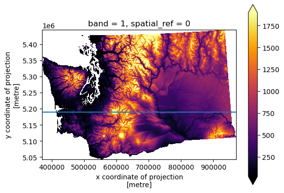
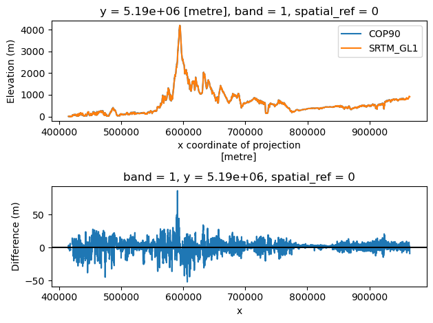
Profile plot

#y=5300000
y=5190000
f, ax = plt.subplots()
cop_xds_wa.plot.imshow(cmap='inferno', robust=True, ax=ax)
ax.set_aspect('equal')
ax.axhline(y)

f, axa = plt.subplots(2, 1)
cop_xds_wa.sel(y=y, method='nearest').plot(ax=axa[0], label='COP90')
srtm_xds_proj.sel(y=y, method='nearest').plot(ax=axa[0], label='SRTM_GL1')
axa[0].legend()
axa[0].set_ylabel('Elevation (m)')
diff.sel(y=y, method='nearest').plot(ax=axa[1])
axa[1].axhline(0, color='k')
axa[1].set_ylabel('Difference (m)')
plt.tight_layout()

Using hvplot

import hvplot.xarray

#Nice for interactive viewing, but results in huge notebook file size
#diff.hvplot(x='x', y='y', cmap='RdBu', clim=(-10,10), aspect='equal')

Part 5: Raster Filtering

• Applying digital filters is a common operation in image processing

• Can be useful to filter outliers, reduce noise, find edges, etc.

• Lots of useful kernel-based filters in scipy.ndimage: https://docs.scipy.org/doc/scipy/reference/ndimage.html

  • Note that many of these do not elegantly handle NaN or masked values!

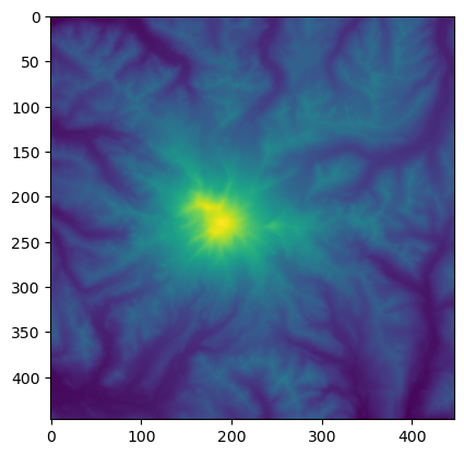
Extract a portion of the DEM around Mt Rainier

#From Raster1 lab
window_bounds = (581385.0, 5174595.0, 612105.0, 5205315.0)
print("Window bounds: ", window_bounds)
window_extent = [window_bounds[0], window_bounds[2], window_bounds[1], window_bounds[3]]
print("Window extent: ", window_extent)

Window bounds:  (581385.0, 5174595.0, 612105.0, 5205315.0)
Window extent:  [581385.0, 612105.0, 5174595.0, 5205315.0]

rainier_window = rio.windows.from_bounds(*window_bounds, transform=src_proj.transform)
rainier_window

Window(col_off=3152.0629486113885, row_off=3495.691051183996, width=446.846299668081, height=446.8462996680755)

rainier_ma = src_proj.read(1, window=rainier_window)
#rainier_ma = np.ma.masked_equal(rainier_ma, src_proj.nodata)

plt.imshow(rainier_ma)

<matplotlib.image.AxesImage at 0x7f552dfd4e80>

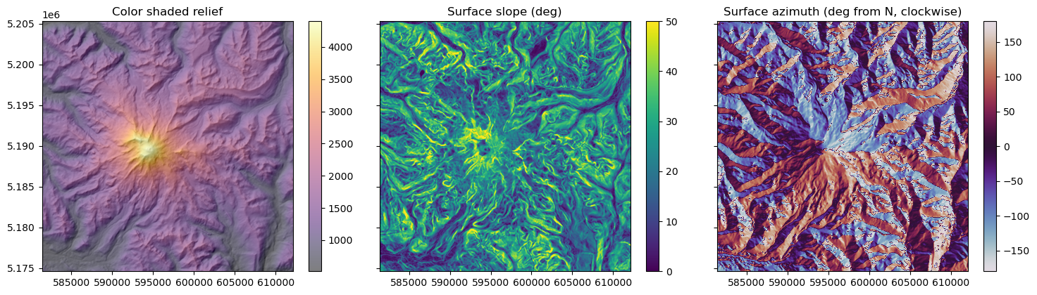
rainier_hs, slope, aspect = hillshade(rainier_ma, src_proj.res[0])
print(slope.max(), aspect.max())

66.14135 179.99565

f, axa = plt.subplots(1, 3, sharex=True, sharey=True, figsize=(15,4))
axa[0].imshow(rainier_hs, extent=window_extent, cmap='gray')
m = axa[0].imshow(rainier_ma, cmap='inferno', extent=window_extent, alpha=0.5)
#axa[1].imshow(hs)
f.colorbar(m, ax=axa[0])
axa[0].set_title('Color shaded relief')
m = axa[1].imshow(slope, extent=window_extent, vmax=50)
f.colorbar(m, ax=axa[1])
axa[1].set_title('Surface slope (deg)')
m = axa[2].imshow(aspect, cmap='twilight', extent=window_extent)
f.colorbar(m, ax=axa[2])
axa[2].set_title('Surface azimuth (deg from N, clockwise)')
plt.tight_layout()

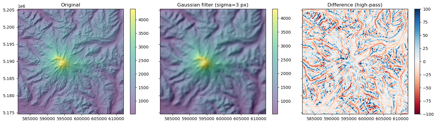
Gaussian smoothing

from scipy.ndimage import gaussian_filter
#This controls width of gaussian kernel standard deviation in pixels
#Play around with a few values
sigma = 3
rainier_ma_smooth = gaussian_filter(rainier_ma, sigma=sigma)
rainier_hs_smooth, slope, aspect = hillshade(rainier_ma_smooth, src_proj.res[0])

f, axa = plt.subplots(1,3, sharex=True, sharey=True, figsize=(15,4))
axa[0].imshow(rainier_hs, extent=window_extent, cmap='gray')
m = axa[0].imshow(rainier_ma, extent=window_extent, alpha=0.5)
f.colorbar(m, ax=axa[0])
axa[0].set_title("Original")
axa[1].imshow(rainier_hs_smooth, extent=window_extent, cmap='gray')
m = axa[1].imshow(rainier_ma_smooth, extent=window_extent, alpha=0.5)
f.colorbar(m, ax=axa[1])
axa[1].set_title("Gaussian filter (sigma=%s px)" % sigma)
m = axa[2].imshow(rainier_ma - rainier_ma_smooth, extent=window_extent, cmap='RdBu', vmin=-100, vmax=100)
f.colorbar(m, ax=axa[2])
axa[2].set_title("Difference (high-pass)")
plt.tight_layout()

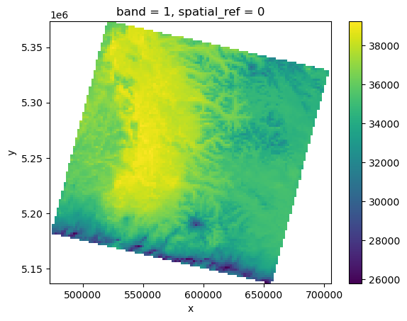
Overviews and COGs

• https://developers.planet.com/docs/planetschool/an-introduction-to-cloud-optimized-geotiffs-cogs-part-1-overview/

• https://gdal.org/programs/gdaladdo.html

• https://gdal.org/drivers/raster/cog.html

#Landsat-8 image is a COG
tir_fn = '../../05_Raster1_GDAL_rasterio_LS8/LS8_sample/LC08_L2SP_046027_20181224_20200829_02_T1_ST_B10.TIF'

!gdalinfo $tir_fn

Driver: GTiff/GeoTIFF
Files: ../../05_Raster1_GDAL_rasterio_LS8/LS8_sample/LC08_L2SP_046027_20181224_20200829_02_T1_ST_B10.TIF
       ../../05_Raster1_GDAL_rasterio_LS8/LS8_sample/LC08_L2SP_046027_20181224_20200829_02_T1_ST_B10.TIF.aux.xml
Size is 7771, 7881
Coordinate System is:
PROJCRS["WGS 84 / UTM zone 10N",
    BASEGEOGCRS["WGS 84",
        DATUM["World Geodetic System 1984",
            ELLIPSOID["WGS 84",6378137,298.257223563,
                LENGTHUNIT["metre",1]]],
        PRIMEM["Greenwich",0,
            ANGLEUNIT["degree",0.0174532925199433]],
        ID["EPSG",4326]],
    CONVERSION["UTM zone 10N",
        METHOD["Transverse Mercator",
            ID["EPSG",9807]],
        PARAMETER["Latitude of natural origin",0,
            ANGLEUNIT["degree",0.0174532925199433],
            ID["EPSG",8801]],
        PARAMETER["Longitude of natural origin",-123,
            ANGLEUNIT["degree",0.0174532925199433],
            ID["EPSG",8802]],
        PARAMETER["Scale factor at natural origin",0.9996,
            SCALEUNIT["unity",1],
            ID["EPSG",8805]],
        PARAMETER["False easting",500000,
            LENGTHUNIT["metre",1],
            ID["EPSG",8806]],
        PARAMETER["False northing",0,
            LENGTHUNIT["metre",1],
            ID["EPSG",8807]]],
    CS[Cartesian,2],
        AXIS["(E)",east,
            ORDER[1],
            LENGTHUNIT["metre",1]],
        AXIS["(N)",north,
            ORDER[2],
            LENGTHUNIT["metre",1]],
    USAGE[
        SCOPE["Engineering survey, topographic mapping."],
        AREA["Between 126°W and 120°W, northern hemisphere between equator and 84°N, onshore and offshore. Canada - British Columbia (BC); Northwest Territories (NWT); Nunavut; Yukon. United States (USA) - Alaska (AK)."],
        BBOX[0,-126,84,-120]],
    ID["EPSG",32610]]
Data axis to CRS axis mapping: 1,2
Origin = (472785.000000000000000,5373315.000000000000000)
Pixel Size = (30.000000000000000,-30.000000000000000)
Metadata:
  AREA_OR_POINT=Point
Image Structure Metadata:
  COMPRESSION=DEFLATE
  INTERLEAVE=BAND
Corner Coordinates:
Upper Left  (  472785.000, 5373315.000) (123d22' 6.59"W, 48d30'44.50"N)
Lower Left  (  472785.000, 5136885.000) (123d21'14.15"W, 46d23' 5.97"N)
Upper Right (  705915.000, 5373315.000) (120d12'48.76"W, 48d28'45.16"N)
Lower Right (  705915.000, 5136885.000) (120d19'24.73"W, 46d21'15.14"N)
Center      (  589350.000, 5255100.000) (121d48'53.62"W, 47d26'35.59"N)
Band 1 Block=256x256 Type=UInt16, ColorInterp=Gray
  Min=23752.000 Max=42219.000 
  Minimum=23752.000, Maximum=42219.000, Mean=35708.987, StdDev=2100.959
  NoData Value=0
  Overviews: 3886x3941, 1943x1971, 972x986, 486x493, 243x247, 122x124
  Metadata:
    STATISTICS_MAXIMUM=42219
    STATISTICS_MEAN=35708.986610756
    STATISTICS_MINIMUM=23752
    STATISTICS_STDDEV=2100.9585113563
    STATISTICS_VALID_PERCENT=66.34

tir = rioxarray.open_rasterio(tir_fn, overview_level=5, mask_and_scale=True).squeeze()
tir

<xarray.DataArray (y: 124, x: 122)>
[15128 values with dtype=float32]
Coordinates:
    band         int64 1
  * x            (x) float64 4.737e+05 4.757e+05 4.776e+05 ... 7.03e+05 7.05e+05
  * y            (y) float64 5.372e+06 5.37e+06 5.369e+06 ... 5.14e+06 5.138e+06
    spatial_ref  int64 0
Attributes:
    AREA_OR_POINT:  Point

xarray.DataArray

• y: 124
• x: 122

• ...

  [15128 values with dtype=float32]

• Coordinates: (4)
  • band
    ()
    int64
    1

    array(1)

  • x
    (x)
    float64
    4.737e+05 4.757e+05 ... 7.05e+05

    array([473740.45082 , 475651.352459, 477562.254098, 479473.155738,
           481384.057377, 483294.959016, 485205.860656, 487116.762295,
           489027.663934, 490938.565574, 492849.467213, 494760.368852,
           496671.270492, 498582.172131, 500493.07377 , 502403.97541 ,
           504314.877049, 506225.778689, 508136.680328, 510047.581967,
           511958.483607, 513869.385246, 515780.286885, 517691.188525,
           519602.090164, 521512.991803, 523423.893443, 525334.795082,
           527245.696721, 529156.598361, 531067.5     , 532978.401639,
           534889.303279, 536800.204918, 538711.106557, 540622.008197,
           542532.909836, 544443.811475, 546354.713115, 548265.614754,
           550176.516393, 552087.418033, 553998.319672, 555909.221311,
           557820.122951, 559731.02459 , 561641.92623 , 563552.827869,
           565463.729508, 567374.631148, 569285.532787, 571196.434426,
           573107.336066, 575018.237705, 576929.139344, 578840.040984,
           580750.942623, 582661.844262, 584572.745902, 586483.647541,
           588394.54918 , 590305.45082 , 592216.352459, 594127.254098,
           596038.155738, 597949.057377, 599859.959016, 601770.860656,
           603681.762295, 605592.663934, 607503.565574, 609414.467213,
           611325.368852, 613236.270492, 615147.172131, 617058.07377 ,
           618968.97541 , 620879.877049, 622790.778689, 624701.680328,
           626612.581967, 628523.483607, 630434.385246, 632345.286885,
           634256.188525, 636167.090164, 638077.991803, 639988.893443,
           641899.795082, 643810.696721, 645721.598361, 647632.5     ,
           649543.401639, 651454.303279, 653365.204918, 655276.106557,
           657187.008197, 659097.909836, 661008.811475, 662919.713115,
           664830.614754, 666741.516393, 668652.418033, 670563.319672,
           672474.221311, 674385.122951, 676296.02459 , 678206.92623 ,
           680117.827869, 682028.729508, 683939.631148, 685850.532787,
           687761.434426, 689672.336066, 691583.237705, 693494.139344,
           695405.040984, 697315.942623, 699226.844262, 701137.745902,
           703048.647541, 704959.54918 ])

  • y
    (y)
    float64
    5.372e+06 5.37e+06 ... 5.138e+06

    array([5372361.653226, 5370454.959677, 5368548.266129, 5366641.572581,
           5364734.879032, 5362828.185484, 5360921.491935, 5359014.798387,
           5357108.104839, 5355201.41129 , 5353294.717742, 5351388.024194,
           5349481.330645, 5347574.637097, 5345667.943548, 5343761.25    ,
           5341854.556452, 5339947.862903, 5338041.169355, 5336134.475806,
           5334227.782258, 5332321.08871 , 5330414.395161, 5328507.701613,
           5326601.008065, 5324694.314516, 5322787.620968, 5320880.927419,
           5318974.233871, 5317067.540323, 5315160.846774, 5313254.153226,
           5311347.459677, 5309440.766129, 5307534.072581, 5305627.379032,
           5303720.685484, 5301813.991935, 5299907.298387, 5298000.604839,
           5296093.91129 , 5294187.217742, 5292280.524194, 5290373.830645,
           5288467.137097, 5286560.443548, 5284653.75    , 5282747.056452,
           5280840.362903, 5278933.669355, 5277026.975806, 5275120.282258,
           5273213.58871 , 5271306.895161, 5269400.201613, 5267493.508065,
           5265586.814516, 5263680.120968, 5261773.427419, 5259866.733871,
           5257960.040323, 5256053.346774, 5254146.653226, 5252239.959677,
           5250333.266129, 5248426.572581, 5246519.879032, 5244613.185484,
           5242706.491935, 5240799.798387, 5238893.104839, 5236986.41129 ,
           5235079.717742, 5233173.024194, 5231266.330645, 5229359.637097,
           5227452.943548, 5225546.25    , 5223639.556452, 5221732.862903,
           5219826.169355, 5217919.475806, 5216012.782258, 5214106.08871 ,
           5212199.395161, 5210292.701613, 5208386.008065, 5206479.314516,
           5204572.620968, 5202665.927419, 5200759.233871, 5198852.540323,
           5196945.846774, 5195039.153226, 5193132.459677, 5191225.766129,
           5189319.072581, 5187412.379032, 5185505.685484, 5183598.991935,
           5181692.298387, 5179785.604839, 5177878.91129 , 5175972.217742,
           5174065.524194, 5172158.830645, 5170252.137097, 5168345.443548,
           5166438.75    , 5164532.056452, 5162625.362903, 5160718.669355,
           5158811.975806, 5156905.282258, 5154998.58871 , 5153091.895161,
           5151185.201613, 5149278.508065, 5147371.814516, 5145465.120968,
           5143558.427419, 5141651.733871, 5139745.040323, 5137838.346774])

  • spatial_ref
    ()
    int64
    0

    crs_wkt :

    PROJCS["WGS 84 / UTM zone 10N",GEOGCS["WGS 84",DATUM["WGS_1984",SPHEROID["WGS 84",6378137,298.257223563,AUTHORITY["EPSG","7030"]],AUTHORITY["EPSG","6326"]],PRIMEM["Greenwich",0,AUTHORITY["EPSG","8901"]],UNIT["degree",0.0174532925199433,AUTHORITY["EPSG","9122"]],AUTHORITY["EPSG","4326"]],PROJECTION["Transverse_Mercator"],PARAMETER["latitude_of_origin",0],PARAMETER["central_meridian",-123],PARAMETER["scale_factor",0.9996],PARAMETER["false_easting",500000],PARAMETER["false_northing",0],UNIT["metre",1,AUTHORITY["EPSG","9001"]],AXIS["Easting",EAST],AXIS["Northing",NORTH],AUTHORITY["EPSG","32610"]]

    semi_major_axis :

    6378137.0

    semi_minor_axis :

    6356752.314245179

    inverse_flattening :

    298.257223563

    reference_ellipsoid_name :

    WGS 84

    longitude_of_prime_meridian :

    0.0

    prime_meridian_name :

    Greenwich

    geographic_crs_name :

    WGS 84

    horizontal_datum_name :

    World Geodetic System 1984

    projected_crs_name :

    WGS 84 / UTM zone 10N

    grid_mapping_name :

    transverse_mercator

    latitude_of_projection_origin :

    0.0

    longitude_of_central_meridian :

    -123.0

    false_easting :

    500000.0

    false_northing :

    0.0

    scale_factor_at_central_meridian :

    0.9996

    spatial_ref :

    PROJCS["WGS 84 / UTM zone 10N",GEOGCS["WGS 84",DATUM["WGS_1984",SPHEROID["WGS 84",6378137,298.257223563,AUTHORITY["EPSG","7030"]],AUTHORITY["EPSG","6326"]],PRIMEM["Greenwich",0,AUTHORITY["EPSG","8901"]],UNIT["degree",0.0174532925199433,AUTHORITY["EPSG","9122"]],AUTHORITY["EPSG","4326"]],PROJECTION["Transverse_Mercator"],PARAMETER["latitude_of_origin",0],PARAMETER["central_meridian",-123],PARAMETER["scale_factor",0.9996],PARAMETER["false_easting",500000],PARAMETER["false_northing",0],UNIT["metre",1,AUTHORITY["EPSG","9001"]],AXIS["Easting",EAST],AXIS["Northing",NORTH],AUTHORITY["EPSG","32610"]]

    GeoTransform :

    472785.0 1910.9016393442623 0.0 5373315.0 0.0 -1906.6935483870968

    array(0)

• Indexes: (2)
  • x
    PandasIndex

    PandasIndex(Float64Index([473740.45081967214, 475651.35245901643, 477562.25409836066,
                  479473.15573770495,  481384.0573770492, 483294.95901639346,
                   485205.8606557377,   487116.762295082, 489027.66393442627,
                   490938.5655737705,
                  ...
                   687761.4344262296,  689672.3360655739,   691583.237704918,
                   693494.1393442623,  695405.0409836066,  697315.9426229508,
                   699226.8442622952,  701137.7459016393,  703048.6475409836,
                   704959.5491803279],
                 dtype='float64', name='x', length=122))

  • y
    PandasIndex

    PandasIndex(Float64Index([5372361.653225807,  5370454.95967742, 5368548.266129033,
                  5366641.572580645, 5364734.879032258, 5362828.185483871,
                  5360921.491935484, 5359014.798387097, 5357108.104838709,
                  5355201.411290322,
                  ...
                  5154998.588709678, 5153091.895161291, 5151185.201612904,
                  5149278.508064516, 5147371.814516129, 5145465.120967742,
                  5143558.427419355, 5141651.733870968,  5139745.04032258,
                  5137838.346774193],
                 dtype='float64', name='y', length=124))

• Attributes: (1)

  AREA_OR_POINT :

  Point

tir.plot.imshow()

<matplotlib.image.AxesImage at 0x7f552dcbb3d0>

Add overviews to an existing GeoTiff

sea_fn = 'SEA_COP30.tif'

#If your file doesn't include overviews
#!gdaladdo -r gauss $sea_fn

#But since we need to reproject, can specify output file format as COG, which will tile, compress and build overviews
sea_fn_proj = 'SEA_COP30_utm.tif'
if not os.path.exists(sea_fn_proj):
    !gdalwarp -of COG -r cubic -t_srs $dst_crs $sea_fn $sea_fn_proj

CPU times: user 326 µs, sys: 113 µs, total: 439 µs
Wall time: 650 µs

!gdalinfo $sea_fn_proj

Driver: GTiff/GeoTIFF
Files: SEA_COP30_utm.tif
Size is 829, 1406
Coordinate System is:
PROJCRS["WGS 84 / UTM zone 10N",
    BASEGEOGCRS["WGS 84",
        DATUM["World Geodetic System 1984",
            ELLIPSOID["WGS 84",6378137,298.257223563,
                LENGTHUNIT["metre",1]]],
        PRIMEM["Greenwich",0,
            ANGLEUNIT["degree",0.0174532925199433]],
        ID["EPSG",4326]],
    CONVERSION["UTM zone 10N",
        METHOD["Transverse Mercator",
            ID["EPSG",9807]],
        PARAMETER["Latitude of natural origin",0,
            ANGLEUNIT["degree",0.0174532925199433],
            ID["EPSG",8801]],
        PARAMETER["Longitude of natural origin",-123,
            ANGLEUNIT["degree",0.0174532925199433],
            ID["EPSG",8802]],
        PARAMETER["Scale factor at natural origin",0.9996,
            SCALEUNIT["unity",1],
            ID["EPSG",8805]],
        PARAMETER["False easting",500000,
            LENGTHUNIT["metre",1],
            ID["EPSG",8806]],
        PARAMETER["False northing",0,
            LENGTHUNIT["metre",1],
            ID["EPSG",8807]]],
    CS[Cartesian,2],
        AXIS["(E)",east,
            ORDER[1],
            LENGTHUNIT["metre",1]],
        AXIS["(N)",north,
            ORDER[2],
            LENGTHUNIT["metre",1]],
    USAGE[
        SCOPE["Engineering survey, topographic mapping."],
        AREA["Between 126°W and 120°W, northern hemisphere between equator and 84°N, onshore and offshore. Canada - British Columbia (BC); Northwest Territories (NWT); Nunavut; Yukon. United States (USA) - Alaska (AK)."],
        BBOX[0,-126,84,-120]],
    ID["EPSG",32610]]
Data axis to CRS axis mapping: 1,2
Origin = (541275.482176973484457,5293506.379035037010908)
Pixel Size = (27.060262602922780,-27.060262602922780)
Metadata:
  AREA_OR_POINT=Area
Image Structure Metadata:
  COMPRESSION=LZW
  INTERLEAVE=BAND
  LAYOUT=COG
Corner Coordinates:
Upper Left  (  541275.482, 5293506.379) (122d26'55.93"W, 47d47'36.93"N)
Lower Left  (  541275.482, 5255459.650) (122d27' 8.84"W, 47d27' 4.58"N)
Upper Right (  563708.440, 5293506.379) (122d 8'57.71"W, 47d47'30.35"N)
Lower Right (  563708.440, 5255459.650) (122d 9'17.63"W, 47d26'58.07"N)
Center      (  552491.961, 5274483.014) (122d18' 5.05"W, 47d37'17.84"N)
Band 1 Block=512x512 Type=Float32, ColorInterp=Gray
  Overviews: 415x703, 208x352, 104x177

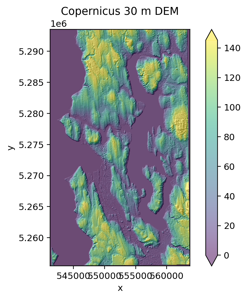
hs_fn = os.path.splitext(sea_fn_proj)[0]+'_hs.tif'

!gdaldem hillshade $sea_fn_proj $hs_fn

0...10...20...30...40...50...60...70...80...90...100 - done.

sea_COP30 = rioxarray.open_rasterio(sea_fn_proj, mask_and_scale=True).squeeze()
sea_COP30_hs = rioxarray.open_rasterio(hs_fn, mask_and_scale=True).squeeze()

f, ax = plt.subplots(dpi=220)
sea_COP30_hs.plot.imshow(ax=ax, cmap='gray', robust=True, add_colorbar=False)
sea_COP30.plot.imshow(ax=ax, cmap='viridis', robust=True, alpha=0.5)
ax.set_aspect('equal')
ax.set_title('Copernicus 30 m DEM');

Some other newer packages worth exploring

Work in Progress: xarray-spatial

• Newer project implementing many raster/DEM analysis functions in Python with Dask/CUDA support

• Uses xarray data model (more complicated than rasterio dataset model)

• https://xarray-spatial.org/

• Surface functions: https://github.com/makepath/xarray-spatial#surface

  • Hillshade: https://xarray-spatial.org/reference/_autosummary/xrspatial.hillshade.hillshade.html#xrspatial.hillshade.hillshade

import xrspatial

#Run the hillshade operation
#hs = xrspatial.hillshade(cop_xds, azimuth=315, angle_altitude=45)
#Note: there are some coordinate scaling and nodata issues here
#hs.plot.imshow(cmap='gray');

xdem

• https://xdem.readthedocs.io/en/latest/quick_start.html