Demo: NumPy, Pandas
Contents
Demo: NumPy, Pandas#
UW Geospatial Data Analysis
CEE467/CEWA567
David Shean
Introduction#
This is a quick demo of some key functionality for these core Python packages, emphasizing topics that will help with lab exercises this week and later in the quarter. It is by no means complete!
Please consult the reading assignment and lists of other excellent, more complete online resources.
NumPy#
NumPy is the fundamental package for scientific computing in Python. It is a Python library that provides a multidimensional array object, various derived objects (such as masked arrays and matrices), and an assortment of routines for fast operations on arrays, including mathematical, logical, shape manipulation, sorting, selecting, I/O, discrete Fourier transforms, basic linear algebra, basic statistical operations, random simulation and much more.
Pandas#
pandas is a fast, powerful, flexible and easy to use open source data analysis and manipulation tool, built on top of the Python programming language.
pandas is a Python package providing fast, flexible, and expressive data structures designed to make working with “relational” or “labeled” data both easy and intuitive. It aims to be the fundamental high-level building block for doing practical, real-world data analysis in Python. Additionally, it has the broader goal of becoming the most powerful and flexible open source data analysis/manipulation tool available in any language. It is already well on its way toward this goal.
Matplotlib#
Matplotlib is a comprehensive library for creating static, animated, and interactive visualizations in Python.
Matplotlib is a Python 2D plotting library which produces publication quality figures in a variety of hardcopy formats and interactive environments across platforms. Matplotlib can be used in Python scripts, the Python and IPython shells, the Jupyter notebook, web application servers, and four graphical user interface toolkits.
Matplotlib tries to make easy things easy and hard things possible. You can generate plots, histograms, power spectra, bar charts, errorcharts, scatterplots, etc., with just a few lines of code. For examples, see the sample plots and thumbnail gallery.
For simple plotting the pyplot module provides a MATLAB-like interface, particularly when combined with IPython. For the power user, you have full control of line styles, font properties, axes properties, etc, via an object oriented interface or via a set of functions familiar to MATLAB users.
Import necessary modules#
Use shorthand, so you don’t have to type out full module name each time
Note different structure for matplotlib package
import numpy as np
import pandas as pd
import matplotlib.pyplot as plt
NumPy 1D array#
#Create 1D array of random integers
#Note parenthesis and brackets
a = np.random.randint(0,10,10)
a
array([3, 9, 4, 6, 5, 4, 4, 3, 9, 1])
type(a)
numpy.ndarray
#np.ndarray?
Constructing an array#
#np.array?
np.array(0, 1, 2)
---------------------------------------------------------------------------
TypeError                                 Traceback (most recent call last)
/tmp/ipykernel_512/449188611.py in <module>
----> 1 np.array(0, 1, 2)

TypeError: array() takes from 1 to 2 positional arguments but 3 were given
#Pass in an array-like object - need brackets around the numbers
np.array([0, 1, 2])
array([0, 1, 2])
mylist = [0, 1, 2]
np.array(mylist)
array([0, 1, 2])
Array properties and datatypes#
a
array([3, 9, 4, 6, 5, 4, 4, 3, 9, 1])
a.shape
(10,)
a.size
10
a.dtype
dtype('int64')
What is ‘int64’?#
Signed integer represented by 64 bits
Each bit can be 0 or 1
0 = 0000000000000000000000000000000000000000000000000000000000000000
1 = 0000000000000000000000000000000000000000000000000000000000000001
2 = 0000000000000000000000000000000000000000000000000000000000000010
…
#Possible unique combinations of 64 bits
range = 2**64
range
18446744073709551616
print(f"{range:.2e}")
1.84e+19
mm = int((2**64)/2)
mm
9223372036854775808
f'A 64-bit signed integer can store values between -{mm} and +{mm}'
'A 64-bit signed integer can store values between -9223372036854775808 and +9223372036854775808'
# Overkill for our single integer values
a
array([3, 9, 4, 6, 5, 4, 4, 3, 9, 1])
#Number of bytes (8 bits each) for each element in the array
a.itemsize
8
#Total number of bytes for 10 elements
a.nbytes
80
# Recast to 8-bit unsigned integer (valid range: 0-255)
b = a.astype('uint8')
b
array([3, 9, 4, 6, 5, 4, 4, 3, 9, 1], dtype=uint8)
b.dtype
dtype('uint8')
2**8
256
b
array([3, 9, 4, 6, 5, 4, 4, 3, 9, 1], dtype=uint8)
b.nbytes
10
#Assign value within valid range
b[0] = 255
b
array([255, 9, 4, 6, 5, 4, 4, 3, 9, 1], dtype=uint8)
#Assign value outside of valid range - overlflow!
# https://en.wikipedia.org/wiki/Integer_overflow
b[0] = 257
b
array([1, 9, 4, 6, 5, 4, 4, 3, 9, 1], dtype=uint8)
2D arrays#
a2 = np.random.random((10,10))
a2
array([[0.52652326, 0.14231249, 0.07566598, 0.59790843, 0.70154418,
        0.52064036, 0.00837979, 0.11927175, 0.13957386, 0.2459467 ],
       [0.6461288 , 0.15507331, 0.90511239, 0.80794971, 0.53618462,
        0.5585833 , 0.37523991, 0.13770533, 0.22708269, 0.79929664],
       [0.32809269, 0.08102169, 0.80168028, 0.2397003 , 0.33923008,
        0.6039445 , 0.06581277, 0.43881912, 0.13918295, 0.81991938],
       [0.54214022, 0.12926722, 0.67341643, 0.97417468, 0.0349868 ,
        0.87610442, 0.24762983, 0.0228108 , 0.5683135 , 0.51484197],
       [0.66986602, 0.12030778, 0.43275939, 0.0487702 , 0.08680747,
        0.77752797, 0.42610501, 0.58918494, 0.24729525, 0.59084971],
       [0.85876637, 0.89397025, 0.96531165, 0.59977053, 0.00839696,
        0.93101856, 0.87715167, 0.79625335, 0.83850491, 0.10052971],
       [0.67171947, 0.35401307, 0.74514409, 0.16502892, 0.30921615,
        0.81304308, 0.074765  , 0.08685205, 0.31914575, 0.23735222],
       [0.47789035, 0.74734751, 0.26285763, 0.59484722, 0.7155864 ,
        0.59474681, 0.47150914, 0.03452718, 0.72332275, 0.47028776],
       [0.02877749, 0.83078924, 0.31289166, 0.30402027, 0.12422959,
        0.5741902 , 0.45545665, 0.8212274 , 0.76181614, 0.108464  ],
       [0.96086507, 0.83894286, 0.84632944, 0.26903294, 0.14547441,
        0.75889114, 0.28676771, 0.36896895, 0.37812949, 0.78041529]])
a2.shape
(10, 10)
a2.size
100
a2.dtype
dtype('float64')
#Get first element along first axis
#Question is this first row or col?
a2[0]
array([0.52652326, 0.14231249, 0.07566598, 0.59790843, 0.70154418,
       0.52064036, 0.00837979, 0.11927175, 0.13957386, 0.2459467 ])
#Get first element along second axis
a2[:,0]
array([0.52652326, 0.6461288 , 0.32809269, 0.54214022, 0.66986602,
       0.85876637, 0.67171947, 0.47789035, 0.02877749, 0.96086507])
#Get first element along both axes
a2[0,0]
0.5265232608453788
#Get slice along first axis - first 3 rows
a2[0:3]
array([[0.52652326, 0.14231249, 0.07566598, 0.59790843, 0.70154418,
        0.52064036, 0.00837979, 0.11927175, 0.13957386, 0.2459467 ],
       [0.6461288 , 0.15507331, 0.90511239, 0.80794971, 0.53618462,
        0.5585833 , 0.37523991, 0.13770533, 0.22708269, 0.79929664],
       [0.32809269, 0.08102169, 0.80168028, 0.2397003 , 0.33923008,
        0.6039445 , 0.06581277, 0.43881912, 0.13918295, 0.81991938]])
#Slice along second axis - first 3 cols
a2[:,0:3]
array([[0.52652326, 0.14231249, 0.07566598],
       [0.6461288 , 0.15507331, 0.90511239],
       [0.32809269, 0.08102169, 0.80168028],
       [0.54214022, 0.12926722, 0.67341643],
       [0.66986602, 0.12030778, 0.43275939],
       [0.85876637, 0.89397025, 0.96531165],
       [0.67171947, 0.35401307, 0.74514409],
       [0.47789035, 0.74734751, 0.26285763],
       [0.02877749, 0.83078924, 0.31289166],
       [0.96086507, 0.83894286, 0.84632944]])
a2[0:3,0:3]
array([[0.52652326, 0.14231249, 0.07566598],
       [0.6461288 , 0.15507331, 0.90511239],
       [0.32809269, 0.08102169, 0.80168028]])
ufunc#
Efficiently perform operation element-by-element in “vectorized” fashion (different than GIS vector dataset)
Do not loop over arrays (unless absolutely necessary)
a2 * 10
array([[5.26523261, 1.42312486, 0.75665984, 5.97908434, 7.01544181,
        5.20640363, 0.08379791, 1.19271753, 1.39573862, 2.459467  ],
       [6.46128797, 1.55073312, 9.05112389, 8.07949708, 5.36184615,
        5.58583304, 3.75239908, 1.37705329, 2.27082693, 7.99296637],
       [3.28092688, 0.8102169 , 8.01680285, 2.39700296, 3.39230084,
        6.03944497, 0.65812771, 4.38819125, 1.3918295 , 8.19919379],
       [5.42140219, 1.2926722 , 6.73416434, 9.74174681, 0.34986796,
        8.76104416, 2.47629829, 0.228108  , 5.68313498, 5.14841969],
       [6.69866023, 1.2030778 , 4.3275939 , 0.48770196, 0.86807469,
        7.77527967, 4.26105014, 5.89184939, 2.47295249, 5.90849707],
       [8.58766372, 8.93970246, 9.65311645, 5.99770527, 0.08396962,
        9.31018559, 8.77151667, 7.96253349, 8.38504906, 1.00529706],
       [6.7171947 , 3.54013069, 7.45144089, 1.65028921, 3.09216152,
        8.13043078, 0.74765   , 0.86852048, 3.1914575 , 2.3735222 ],
       [4.77890351, 7.47347509, 2.62857634, 5.94847221, 7.15586397,
        5.94746812, 4.71509138, 0.34527179, 7.23322755, 4.70287758],
       [0.28777487, 8.30789238, 3.1289166 , 3.04020265, 1.24229588,
        5.741902  , 4.5545665 , 8.21227395, 7.61816135, 1.08463997],
       [9.60865071, 8.38942857, 8.46329441, 2.69032942, 1.45474407,
        7.58891143, 2.86767713, 3.6896895 , 3.78129487, 7.80415291]])
# Don't do this!
#for n, i in enumerate(a2):
#    a2[n] = i + 10
#np.power(a2, 2)
a2**2
array([[2.77226744e-01, 2.02528438e-02, 5.72534107e-03, 3.57494495e-01,
        4.92164238e-01, 2.71066388e-01, 7.02209035e-05, 1.42257512e-02,
        1.94808630e-02, 6.04897792e-02],
       [4.17482422e-01, 2.40477320e-02, 8.19228437e-01, 6.52782731e-01,
        2.87493942e-01, 3.12015307e-01, 1.40804989e-01, 1.89627575e-02,
        5.15665493e-02, 6.38875114e-01],
       [1.07644812e-01, 6.56451420e-03, 6.42691279e-01, 5.74562317e-02,
        1.15077050e-01, 3.64748955e-01, 4.33132086e-03, 1.92562224e-01,
        1.93718936e-02, 6.72267787e-01],
       [2.93916017e-01, 1.67100142e-02, 4.53489693e-01, 9.49016309e-01,
        1.22407590e-03, 7.67558948e-01, 6.13205320e-02, 5.20332575e-04,
        3.22980232e-01, 2.65062253e-01],
       [4.48720489e-01, 1.44739619e-02, 1.87280690e-01, 2.37853201e-03,
        7.53553662e-03, 6.04549740e-01, 1.81565483e-01, 3.47138893e-01,
        6.11549402e-02, 3.49103376e-01],
       [7.37479681e-01, 7.99182800e-01, 9.31826572e-01, 3.59724685e-01,
        7.05089649e-05, 8.66795558e-01, 7.69395047e-01, 6.34019395e-01,
        7.03090478e-01, 1.01062218e-02],
       [4.51207047e-01, 1.25325253e-01, 5.55239714e-01, 2.72345449e-02,
        9.56146285e-02, 6.61039047e-01, 5.58980528e-03, 7.54327828e-03,
        1.01854010e-01, 5.63360766e-02],
       [2.28379187e-01, 5.58528300e-01, 6.90941356e-02, 3.53843216e-01,
        5.12063892e-01, 3.53723770e-01, 2.22320868e-01, 1.19212608e-03,
        5.23195808e-01, 2.21170575e-01],
       [8.28143736e-04, 6.90210757e-01, 9.79011906e-02, 9.24283216e-02,
        1.54329906e-02, 3.29694386e-01, 2.07440760e-01, 6.74414434e-01,
        5.80363824e-01, 1.17644387e-02],
       [9.23261684e-01, 7.03825118e-01, 7.16273522e-01, 7.23787240e-02,
        2.11628030e-02, 5.75915767e-01, 8.22357214e-02, 1.36138086e-01,
        1.42981909e-01, 6.09048026e-01]])
#a2**0.5
np.sqrt(a2)
array([[0.72561923, 0.37724327, 0.27507451, 0.77324539, 0.83758234,
        0.72155413, 0.0915412 , 0.34535743, 0.37359585, 0.49593014],
       [0.80382137, 0.39379349, 0.95137395, 0.89886023, 0.73224628,
        0.74738431, 0.61256829, 0.37108669, 0.47653194, 0.89403391],
       [0.57279376, 0.28464309, 0.89536601, 0.48959197, 0.58243462,
        0.77713866, 0.25654   , 0.66243424, 0.37307231, 0.905494  ],
       [0.73630172, 0.35953751, 0.82061954, 0.98700288, 0.18704758,
        0.9360045 , 0.49762418, 0.15103245, 0.7538657 , 0.71752489],
       [0.81845343, 0.34685412, 0.6578445 , 0.22083975, 0.29463107,
        0.88177546, 0.6527672 , 0.76758383, 0.49728789, 0.76866749],
       [0.92669648, 0.9455    , 0.98250275, 0.77444853, 0.09163494,
        0.96489303, 0.93656375, 0.89233029, 0.91569914, 0.3170642 ],
       [0.81958494, 0.59498997, 0.86321729, 0.40623752, 0.55607207,
        0.90168901, 0.27343189, 0.29470672, 0.56492986, 0.48718808],
       [0.69129614, 0.86449263, 0.51269643, 0.77126339, 0.8459234 ,
        0.7711983 , 0.68666523, 0.1858149 , 0.85048384, 0.6857753 ],
       [0.16963928, 0.91147641, 0.5593672 , 0.55138033, 0.35246218,
        0.75775339, 0.67487528, 0.90621598, 0.87282079, 0.32933873],
       [0.98023725, 0.91593824, 0.91996165, 0.51868386, 0.38141107,
        0.87114358, 0.53550697, 0.60742814, 0.61492234, 0.88341117]])
Built-in functions#
Operate over entire array, specified axes, or slice
Very fast/efficient
a2.mean()
0.46351243272781467
a2.std()
0.2922564296409726
a2.min()
0.008379791373509304
a2
array([[0.52652326, 0.14231249, 0.07566598, 0.59790843, 0.70154418,
        0.52064036, 0.00837979, 0.11927175, 0.13957386, 0.2459467 ],
       [0.6461288 , 0.15507331, 0.90511239, 0.80794971, 0.53618462,
        0.5585833 , 0.37523991, 0.13770533, 0.22708269, 0.79929664],
       [0.32809269, 0.08102169, 0.80168028, 0.2397003 , 0.33923008,
        0.6039445 , 0.06581277, 0.43881912, 0.13918295, 0.81991938],
       [0.54214022, 0.12926722, 0.67341643, 0.97417468, 0.0349868 ,
        0.87610442, 0.24762983, 0.0228108 , 0.5683135 , 0.51484197],
       [0.66986602, 0.12030778, 0.43275939, 0.0487702 , 0.08680747,
        0.77752797, 0.42610501, 0.58918494, 0.24729525, 0.59084971],
       [0.85876637, 0.89397025, 0.96531165, 0.59977053, 0.00839696,
        0.93101856, 0.87715167, 0.79625335, 0.83850491, 0.10052971],
       [0.67171947, 0.35401307, 0.74514409, 0.16502892, 0.30921615,
        0.81304308, 0.074765  , 0.08685205, 0.31914575, 0.23735222],
       [0.47789035, 0.74734751, 0.26285763, 0.59484722, 0.7155864 ,
        0.59474681, 0.47150914, 0.03452718, 0.72332275, 0.47028776],
       [0.02877749, 0.83078924, 0.31289166, 0.30402027, 0.12422959,
        0.5741902 , 0.45545665, 0.8212274 , 0.76181614, 0.108464  ],
       [0.96086507, 0.83894286, 0.84632944, 0.26903294, 0.14547441,
        0.75889114, 0.28676771, 0.36896895, 0.37812949, 0.78041529]])
Note on axis order#
When indexing, first axis (0) will extract rows, second axis (1) will extract cols
When aggregating (e.g., computing mean along an axis), you are specifing the dimension of the array that will be collapsed, not the dimension that will be returned
So axis=0 will aggregate values across all rows for each column in a 2D array
a2[0:3,0:3]
array([[0.52652326, 0.14231249, 0.07566598],
       [0.6461288 , 0.15507331, 0.90511239],
       [0.32809269, 0.08102169, 0.80168028]])
a2[0:3,0:3].min(axis=0)
array([0.32809269, 0.08102169, 0.07566598])
a2[0:3,0:3].min(axis=1)
array([0.07566598, 0.15507331, 0.08102169])
Basic array plotting and visualization#
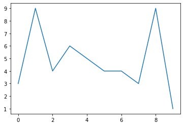
a
array([3, 9, 4, 6, 5, 4, 4, 3, 9, 1])
plt.plot(a)
[<matplotlib.lines.Line2D at 0x7f7d7cd5f160>]
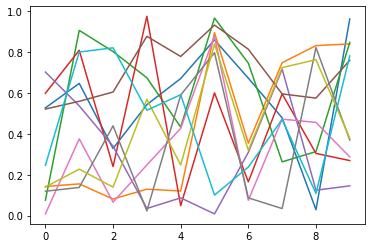
a2
array([[0.52652326, 0.14231249, 0.07566598, 0.59790843, 0.70154418,
        0.52064036, 0.00837979, 0.11927175, 0.13957386, 0.2459467 ],
       [0.6461288 , 0.15507331, 0.90511239, 0.80794971, 0.53618462,
        0.5585833 , 0.37523991, 0.13770533, 0.22708269, 0.79929664],
       [0.32809269, 0.08102169, 0.80168028, 0.2397003 , 0.33923008,
        0.6039445 , 0.06581277, 0.43881912, 0.13918295, 0.81991938],
       [0.54214022, 0.12926722, 0.67341643, 0.97417468, 0.0349868 ,
        0.87610442, 0.24762983, 0.0228108 , 0.5683135 , 0.51484197],
       [0.66986602, 0.12030778, 0.43275939, 0.0487702 , 0.08680747,
        0.77752797, 0.42610501, 0.58918494, 0.24729525, 0.59084971],
       [0.85876637, 0.89397025, 0.96531165, 0.59977053, 0.00839696,
        0.93101856, 0.87715167, 0.79625335, 0.83850491, 0.10052971],
       [0.67171947, 0.35401307, 0.74514409, 0.16502892, 0.30921615,
        0.81304308, 0.074765  , 0.08685205, 0.31914575, 0.23735222],
       [0.47789035, 0.74734751, 0.26285763, 0.59484722, 0.7155864 ,
        0.59474681, 0.47150914, 0.03452718, 0.72332275, 0.47028776],
       [0.02877749, 0.83078924, 0.31289166, 0.30402027, 0.12422959,
        0.5741902 , 0.45545665, 0.8212274 , 0.76181614, 0.108464  ],
       [0.96086507, 0.83894286, 0.84632944, 0.26903294, 0.14547441,
        0.75889114, 0.28676771, 0.36896895, 0.37812949, 0.78041529]])
plt.plot(a2)
[<matplotlib.lines.Line2D at 0x7f7d7cbd3f10>,
 <matplotlib.lines.Line2D at 0x7f7d7cbd3f70>,
 <matplotlib.lines.Line2D at 0x7f7d7cb610d0>,
 <matplotlib.lines.Line2D at 0x7f7d7cb611f0>,
 <matplotlib.lines.Line2D at 0x7f7d7cb61310>,
 <matplotlib.lines.Line2D at 0x7f7d7cb61430>,
 <matplotlib.lines.Line2D at 0x7f7d7cb61550>,
 <matplotlib.lines.Line2D at 0x7f7d7cb61670>,
 <matplotlib.lines.Line2D at 0x7f7d7cb61790>,
 <matplotlib.lines.Line2D at 0x7f7d7cb618b0>]
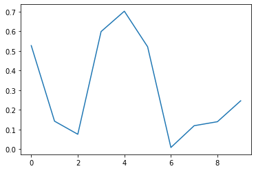
plt.plot(a2[0])
[<matplotlib.lines.Line2D at 0x7f7d7cb5dd60>]
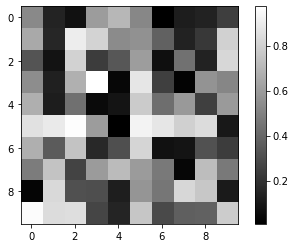
#2D array visualization
plt.imshow(a2, cmap='gray')
plt.colorbar()
<matplotlib.colorbar.Colorbar at 0x7f7d7c27b4f0>
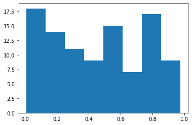
plt.hist(a2.ravel(), bins='auto')
(array([18., 14., 11.,  9., 15.,  7., 17.,  9.]),
 array([0.00837979, 0.12910415, 0.24982851, 0.37055287, 0.49127724,
        0.6120016 , 0.73272596, 0.85345032, 0.97417468]),
 <BarContainer object of 8 artists>)
Boolean arrays and fancy indexing#
a2
array([[0.52652326, 0.14231249, 0.07566598, 0.59790843, 0.70154418,
        0.52064036, 0.00837979, 0.11927175, 0.13957386, 0.2459467 ],
       [0.6461288 , 0.15507331, 0.90511239, 0.80794971, 0.53618462,
        0.5585833 , 0.37523991, 0.13770533, 0.22708269, 0.79929664],
       [0.32809269, 0.08102169, 0.80168028, 0.2397003 , 0.33923008,
        0.6039445 , 0.06581277, 0.43881912, 0.13918295, 0.81991938],
       [0.54214022, 0.12926722, 0.67341643, 0.97417468, 0.0349868 ,
        0.87610442, 0.24762983, 0.0228108 , 0.5683135 , 0.51484197],
       [0.66986602, 0.12030778, 0.43275939, 0.0487702 , 0.08680747,
        0.77752797, 0.42610501, 0.58918494, 0.24729525, 0.59084971],
       [0.85876637, 0.89397025, 0.96531165, 0.59977053, 0.00839696,
        0.93101856, 0.87715167, 0.79625335, 0.83850491, 0.10052971],
       [0.67171947, 0.35401307, 0.74514409, 0.16502892, 0.30921615,
        0.81304308, 0.074765  , 0.08685205, 0.31914575, 0.23735222],
       [0.47789035, 0.74734751, 0.26285763, 0.59484722, 0.7155864 ,
        0.59474681, 0.47150914, 0.03452718, 0.72332275, 0.47028776],
       [0.02877749, 0.83078924, 0.31289166, 0.30402027, 0.12422959,
        0.5741902 , 0.45545665, 0.8212274 , 0.76181614, 0.108464  ],
       [0.96086507, 0.83894286, 0.84632944, 0.26903294, 0.14547441,
        0.75889114, 0.28676771, 0.36896895, 0.37812949, 0.78041529]])
a2 > 0.5
array([[ True, False, False,  True,  True,  True, False, False, False,
        False],
       [ True, False,  True,  True,  True,  True, False, False, False,
         True],
       [False, False,  True, False, False,  True, False, False, False,
         True],
       [ True, False,  True,  True, False,  True, False, False,  True,
         True],
       [ True, False, False, False, False,  True, False,  True, False,
         True],
       [ True,  True,  True,  True, False,  True,  True,  True,  True,
        False],
       [ True, False,  True, False, False,  True, False, False, False,
        False],
       [False,  True, False,  True,  True,  True, False, False,  True,
        False],
       [False,  True, False, False, False,  True, False,  True,  True,
        False],
       [ True,  True,  True, False, False,  True, False, False, False,
         True]])
idx = (a2 > 0.5)
idx
array([[ True, False, False,  True,  True,  True, False, False, False,
        False],
       [ True, False,  True,  True,  True,  True, False, False, False,
         True],
       [False, False,  True, False, False,  True, False, False, False,
         True],
       [ True, False,  True,  True, False,  True, False, False,  True,
         True],
       [ True, False, False, False, False,  True, False,  True, False,
         True],
       [ True,  True,  True,  True, False,  True,  True,  True,  True,
        False],
       [ True, False,  True, False, False,  True, False, False, False,
        False],
       [False,  True, False,  True,  True,  True, False, False,  True,
        False],
       [False,  True, False, False, False,  True, False,  True,  True,
        False],
       [ True,  True,  True, False, False,  True, False, False, False,
         True]])
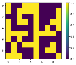
# Quick visualization, True = yellow (1)
plt.imshow(idx)
plt.colorbar()
<matplotlib.colorbar.Colorbar at 0x7f7d7c13b910>
# Return only elements where condition is True
a2[idx]
array([0.52652326, 0.59790843, 0.70154418, 0.52064036, 0.6461288 ,
       0.90511239, 0.80794971, 0.53618462, 0.5585833 , 0.79929664,
       0.80168028, 0.6039445 , 0.81991938, 0.54214022, 0.67341643,
       0.97417468, 0.87610442, 0.5683135 , 0.51484197, 0.66986602,
       0.77752797, 0.58918494, 0.59084971, 0.85876637, 0.89397025,
       0.96531165, 0.59977053, 0.93101856, 0.87715167, 0.79625335,
       0.83850491, 0.67171947, 0.74514409, 0.81304308, 0.74734751,
       0.59484722, 0.7155864 , 0.59474681, 0.72332275, 0.83078924,
       0.5741902 , 0.8212274 , 0.76181614, 0.96086507, 0.83894286,
       0.84632944, 0.75889114, 0.78041529])
# Original shape
a2.shape
(10, 10)
# Selected shape
a2[idx].shape
#idx.nonzero()[0].size
(48,)
#Can also be used for assignment
#a2[idx] = 0
### Bitwise operators, combining boolean arrays
(a2 > 0.5)
array([[ True, False, False,  True,  True,  True, False, False, False,
        False],
       [ True, False,  True,  True,  True,  True, False, False, False,
         True],
       [False, False,  True, False, False,  True, False, False, False,
         True],
       [ True, False,  True,  True, False,  True, False, False,  True,
         True],
       [ True, False, False, False, False,  True, False,  True, False,
         True],
       [ True,  True,  True,  True, False,  True,  True,  True,  True,
        False],
       [ True, False,  True, False, False,  True, False, False, False,
        False],
       [False,  True, False,  True,  True,  True, False, False,  True,
        False],
       [False,  True, False, False, False,  True, False,  True,  True,
        False],
       [ True,  True,  True, False, False,  True, False, False, False,
         True]])
(a2 < 0.7)
array([[ True,  True,  True,  True, False,  True,  True,  True,  True,
         True],
       [ True,  True, False, False,  True,  True,  True,  True,  True,
        False],
       [ True,  True, False,  True,  True,  True,  True,  True,  True,
        False],
       [ True,  True,  True, False,  True, False,  True,  True,  True,
         True],
       [ True,  True,  True,  True,  True, False,  True,  True,  True,
         True],
       [False, False, False,  True,  True, False, False, False, False,
         True],
       [ True,  True, False,  True,  True, False,  True,  True,  True,
         True],
       [ True, False,  True,  True, False,  True,  True,  True, False,
         True],
       [ True, False,  True,  True,  True,  True,  True, False, False,
         True],
       [False, False, False,  True,  True, False,  True,  True,  True,
        False]])
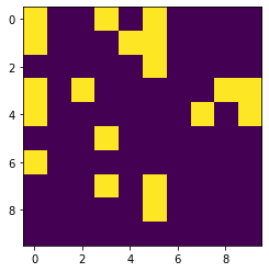
#Bitwise and - True if both are True
idx = (a2 > 0.5) & (a2 < 0.7)
#Bitwise or - True if either is True
#idx = (a < 0.5) | (a > 0.9)
idx
array([[ True, False, False,  True, False,  True, False, False, False,
        False],
       [ True, False, False, False,  True,  True, False, False, False,
        False],
       [False, False, False, False, False,  True, False, False, False,
        False],
       [ True, False,  True, False, False, False, False, False,  True,
         True],
       [ True, False, False, False, False, False, False,  True, False,
         True],
       [False, False, False,  True, False, False, False, False, False,
        False],
       [ True, False, False, False, False, False, False, False, False,
        False],
       [False, False, False,  True, False,  True, False, False, False,
        False],
       [False, False, False, False, False,  True, False, False, False,
        False],
       [False, False, False, False, False, False, False, False, False,
        False]])
plt.imshow(idx)
<matplotlib.image.AxesImage at 0x7f7d7c0c5700>

a2[idx]
array([0.52652326, 0.59790843, 0.52064036, 0.6461288 , 0.53618462,
       0.5585833 , 0.6039445 , 0.54214022, 0.67341643, 0.5683135 ,
       0.51484197, 0.66986602, 0.58918494, 0.59084971, 0.59977053,
       0.67171947, 0.59484722, 0.59474681, 0.5741902 ])
a2[idx].shape
(19,)
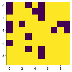
#Invert the boolean array
~idx
array([[False,  True,  True, False,  True, False,  True,  True,  True,
         True],
       [False,  True,  True,  True, False, False,  True,  True,  True,
         True],
       [ True,  True,  True,  True,  True, False,  True,  True,  True,
         True],
       [False,  True, False,  True,  True,  True,  True,  True, False,
        False],
       [False,  True,  True,  True,  True,  True,  True, False,  True,
        False],
       [ True,  True,  True, False,  True,  True,  True,  True,  True,
         True],
       [False,  True,  True,  True,  True,  True,  True,  True,  True,
         True],
       [ True,  True,  True, False,  True, False,  True,  True,  True,
         True],
       [ True,  True,  True,  True,  True, False,  True,  True,  True,
         True],
       [ True,  True,  True,  True,  True,  True,  True,  True,  True,
         True]])
plt.imshow(idx)
<matplotlib.image.AxesImage at 0x7f7d7c0b99a0>
plt.imshow(~idx)
<matplotlib.image.AxesImage at 0x7f7d7c0fdbe0>
a2[~idx].shape
(81,)
Masked array#
a2
array([[0.52652326, 0.14231249, 0.07566598, 0.59790843, 0.70154418,
        0.52064036, 0.00837979, 0.11927175, 0.13957386, 0.2459467 ],
       [0.6461288 , 0.15507331, 0.90511239, 0.80794971, 0.53618462,
        0.5585833 , 0.37523991, 0.13770533, 0.22708269, 0.79929664],
       [0.32809269, 0.08102169, 0.80168028, 0.2397003 , 0.33923008,
        0.6039445 , 0.06581277, 0.43881912, 0.13918295, 0.81991938],
       [0.54214022, 0.12926722, 0.67341643, 0.97417468, 0.0349868 ,
        0.87610442, 0.24762983, 0.0228108 , 0.5683135 , 0.51484197],
       [0.66986602, 0.12030778, 0.43275939, 0.0487702 , 0.08680747,
        0.77752797, 0.42610501, 0.58918494, 0.24729525, 0.59084971],
       [0.85876637, 0.89397025, 0.96531165, 0.59977053, 0.00839696,
        0.93101856, 0.87715167, 0.79625335, 0.83850491, 0.10052971],
       [0.67171947, 0.35401307, 0.74514409, 0.16502892, 0.30921615,
        0.81304308, 0.074765  , 0.08685205, 0.31914575, 0.23735222],
       [0.47789035, 0.74734751, 0.26285763, 0.59484722, 0.7155864 ,
        0.59474681, 0.47150914, 0.03452718, 0.72332275, 0.47028776],
       [0.02877749, 0.83078924, 0.31289166, 0.30402027, 0.12422959,
        0.5741902 , 0.45545665, 0.8212274 , 0.76181614, 0.108464  ],
       [0.96086507, 0.83894286, 0.84632944, 0.26903294, 0.14547441,
        0.75889114, 0.28676771, 0.36896895, 0.37812949, 0.78041529]])
idx
array([[ True, False, False,  True, False,  True, False, False, False,
        False],
       [ True, False, False, False,  True,  True, False, False, False,
        False],
       [False, False, False, False, False,  True, False, False, False,
        False],
       [ True, False,  True, False, False, False, False, False,  True,
         True],
       [ True, False, False, False, False, False, False,  True, False,
         True],
       [False, False, False,  True, False, False, False, False, False,
        False],
       [ True, False, False, False, False, False, False, False, False,
        False],
       [False, False, False,  True, False,  True, False, False, False,
        False],
       [False, False, False, False, False,  True, False, False, False,
        False],
       [False, False, False, False, False, False, False, False, False,
        False]])
#np.ma.array
ma = np.ma.array(a2, mask=~idx)
ma
masked_array(
  data=[[0.5265232608453788, --, --, 0.5979084337784969, --,
         0.5206403629685025, --, --, --, --],
        [0.6461287968711238, --, --, --, 0.5361846154058071,
         0.558583303937883, --, --, --, --],
        [--, --, --, --, --, 0.6039444969658847, --, --, --, --],
        [0.5421402189101205, --, 0.6734164335026674, --, --, --, --, --,
         0.5683134980882404, 0.5148419689595748],
        [0.6698660228152108, --, --, --, --, --, --, 0.5891849393173709,
         --, 0.5908497065541548],
        [--, --, --, 0.5997705271856745, --, --, --, --, --, --],
        [0.6717194703376138, --, --, --, --, --, --, --, --, --],
        [--, --, --, 0.5948472205118084, --, 0.594746811681392, --, --,
         --, --],
        [--, --, --, --, --, 0.5741901997787556, --, --, --, --],
        [--, --, --, --, --, --, --, --, --, --]],
  mask=[[False,  True,  True, False,  True, False,  True,  True,  True,
          True],
        [False,  True,  True,  True, False, False,  True,  True,  True,
          True],
        [ True,  True,  True,  True,  True, False,  True,  True,  True,
          True],
        [False,  True, False,  True,  True,  True,  True,  True, False,
         False],
        [False,  True,  True,  True,  True,  True,  True, False,  True,
         False],
        [ True,  True,  True, False,  True,  True,  True,  True,  True,
          True],
        [False,  True,  True,  True,  True,  True,  True,  True,  True,
          True],
        [ True,  True,  True, False,  True, False,  True,  True,  True,
          True],
        [ True,  True,  True,  True,  True, False,  True,  True,  True,
          True],
        [ True,  True,  True,  True,  True,  True,  True,  True,  True,
          True]],
  fill_value=1e+20)
a2.mean()
0.46351243272781467
ma.mean()
0.5880947520218769
plt.imshow(ma)
<matplotlib.image.AxesImage at 0x7f7d7c1bceb0>
Masked array vs. np.nan#
We will come back to this in Lab05
Useful for representing nodata in raster datasets
Useful for dynamically masking outliers for calculations without removing values or creating new arrays
np.nan is float32 or float64, so if your original array is int8, much more efficient to use additional 1-bit mask than cast everything as float32
Pandas!#
#pd.DataFrame?
df = pd.DataFrame(a2)
df
| 0 | 1 | 2 | 3 | 4 | 5 | 6 | 7 | 8 | 9 | |
|---|---|---|---|---|---|---|---|---|---|---|
| 0 | 0.526523 | 0.142312 | 0.075666 | 0.597908 | 0.701544 | 0.520640 | 0.008380 | 0.119272 | 0.139574 | 0.245947 |
| 1 | 0.646129 | 0.155073 | 0.905112 | 0.807950 | 0.536185 | 0.558583 | 0.375240 | 0.137705 | 0.227083 | 0.799297 |
| 2 | 0.328093 | 0.081022 | 0.801680 | 0.239700 | 0.339230 | 0.603944 | 0.065813 | 0.438819 | 0.139183 | 0.819919 |
| 3 | 0.542140 | 0.129267 | 0.673416 | 0.974175 | 0.034987 | 0.876104 | 0.247630 | 0.022811 | 0.568313 | 0.514842 |
| 4 | 0.669866 | 0.120308 | 0.432759 | 0.048770 | 0.086807 | 0.777528 | 0.426105 | 0.589185 | 0.247295 | 0.590850 |
| 5 | 0.858766 | 0.893970 | 0.965312 | 0.599771 | 0.008397 | 0.931019 | 0.877152 | 0.796253 | 0.838505 | 0.100530 |
| 6 | 0.671719 | 0.354013 | 0.745144 | 0.165029 | 0.309216 | 0.813043 | 0.074765 | 0.086852 | 0.319146 | 0.237352 |
| 7 | 0.477890 | 0.747348 | 0.262858 | 0.594847 | 0.715586 | 0.594747 | 0.471509 | 0.034527 | 0.723323 | 0.470288 |
| 8 | 0.028777 | 0.830789 | 0.312892 | 0.304020 | 0.124230 | 0.574190 | 0.455457 | 0.821227 | 0.761816 | 0.108464 |
| 9 | 0.960865 | 0.838943 | 0.846329 | 0.269033 | 0.145474 | 0.758891 | 0.286768 | 0.368969 | 0.378129 | 0.780415 |
df.index = ['a','b','c','d','e','f','g','h','i','j']
df
| 0 | 1 | 2 | 3 | 4 | 5 | 6 | 7 | 8 | 9 | |
|---|---|---|---|---|---|---|---|---|---|---|
| a | 0.526523 | 0.142312 | 0.075666 | 0.597908 | 0.701544 | 0.520640 | 0.008380 | 0.119272 | 0.139574 | 0.245947 |
| b | 0.646129 | 0.155073 | 0.905112 | 0.807950 | 0.536185 | 0.558583 | 0.375240 | 0.137705 | 0.227083 | 0.799297 |
| c | 0.328093 | 0.081022 | 0.801680 | 0.239700 | 0.339230 | 0.603944 | 0.065813 | 0.438819 | 0.139183 | 0.819919 |
| d | 0.542140 | 0.129267 | 0.673416 | 0.974175 | 0.034987 | 0.876104 | 0.247630 | 0.022811 | 0.568313 | 0.514842 |
| e | 0.669866 | 0.120308 | 0.432759 | 0.048770 | 0.086807 | 0.777528 | 0.426105 | 0.589185 | 0.247295 | 0.590850 |
| f | 0.858766 | 0.893970 | 0.965312 | 0.599771 | 0.008397 | 0.931019 | 0.877152 | 0.796253 | 0.838505 | 0.100530 |
| g | 0.671719 | 0.354013 | 0.745144 | 0.165029 | 0.309216 | 0.813043 | 0.074765 | 0.086852 | 0.319146 | 0.237352 |
| h | 0.477890 | 0.747348 | 0.262858 | 0.594847 | 0.715586 | 0.594747 | 0.471509 | 0.034527 | 0.723323 | 0.470288 |
| i | 0.028777 | 0.830789 | 0.312892 | 0.304020 | 0.124230 | 0.574190 | 0.455457 | 0.821227 | 0.761816 | 0.108464 |
| j | 0.960865 | 0.838943 | 0.846329 | 0.269033 | 0.145474 | 0.758891 | 0.286768 | 0.368969 | 0.378129 | 0.780415 |
# Still just NumPy array under the hood
df.values
array([[0.52652326, 0.14231249, 0.07566598, 0.59790843, 0.70154418,
        0.52064036, 0.00837979, 0.11927175, 0.13957386, 0.2459467 ],
       [0.6461288 , 0.15507331, 0.90511239, 0.80794971, 0.53618462,
        0.5585833 , 0.37523991, 0.13770533, 0.22708269, 0.79929664],
       [0.32809269, 0.08102169, 0.80168028, 0.2397003 , 0.33923008,
        0.6039445 , 0.06581277, 0.43881912, 0.13918295, 0.81991938],
       [0.54214022, 0.12926722, 0.67341643, 0.97417468, 0.0349868 ,
        0.87610442, 0.24762983, 0.0228108 , 0.5683135 , 0.51484197],
       [0.66986602, 0.12030778, 0.43275939, 0.0487702 , 0.08680747,
        0.77752797, 0.42610501, 0.58918494, 0.24729525, 0.59084971],
       [0.85876637, 0.89397025, 0.96531165, 0.59977053, 0.00839696,
        0.93101856, 0.87715167, 0.79625335, 0.83850491, 0.10052971],
       [0.67171947, 0.35401307, 0.74514409, 0.16502892, 0.30921615,
        0.81304308, 0.074765  , 0.08685205, 0.31914575, 0.23735222],
       [0.47789035, 0.74734751, 0.26285763, 0.59484722, 0.7155864 ,
        0.59474681, 0.47150914, 0.03452718, 0.72332275, 0.47028776],
       [0.02877749, 0.83078924, 0.31289166, 0.30402027, 0.12422959,
        0.5741902 , 0.45545665, 0.8212274 , 0.76181614, 0.108464  ],
       [0.96086507, 0.83894286, 0.84632944, 0.26903294, 0.14547441,
        0.75889114, 0.28676771, 0.36896895, 0.37812949, 0.78041529]])
df.index.values
array(['a', 'b', 'c', 'd', 'e', 'f', 'g', 'h', 'i', 'j'], dtype=object)
# Mean of each column
df.mean()
0    0.571077
1    0.429305
2    0.602117
3    0.460120
4    0.300166
5    0.700869
6    0.328882
7    0.341562
8    0.434237
9    0.466790
dtype: float64
# Mean of each row
df.mean(axis=1)
a    0.307777
b    0.514836
c    0.385740
d    0.458369
e    0.398947
f    0.686967
g    0.377628
h    0.509292
i    0.432186
j    0.563382
dtype: float64
Reading files with Pandas#
Most of the time, you will read in tabular data and let Pandas do the work
# Relative path to csv from Lab01
csv_fn = '../01_Shell_Github/data/GLAH14_tllz_conus_lulcfilt_demfilt.csv'
# Quick check using shell `head` command
!head -n 5 $csv_fn
decyear,ordinal,lat,lon,glas_z,dem_z,dem_z_std,lulc
2003.13957078,731266.9433448168,44.157897,-105.356562,1398.51,1400.52,0.33,31
2003.13957081,731266.9433462636,44.150175,-105.358116,1387.11,1384.64,0.43,31
2003.13957081,731266.9433465529,44.148632,-105.358427,1392.83,1383.49,0.28,31
2003.13957081,731266.9433468423,44.147087,-105.358738,1384.24,1382.85,0.84,31
pd.read_csv(csv_fn)
| decyear | ordinal | lat | lon | glas_z | dem_z | dem_z_std | lulc | |
|---|---|---|---|---|---|---|---|---|
| 0 | 2003.139571 | 731266.943345 | 44.157897 | -105.356562 | 1398.51 | 1400.52 | 0.33 | 31 |
| 1 | 2003.139571 | 731266.943346 | 44.150175 | -105.358116 | 1387.11 | 1384.64 | 0.43 | 31 |
| 2 | 2003.139571 | 731266.943347 | 44.148632 | -105.358427 | 1392.83 | 1383.49 | 0.28 | 31 |
| 3 | 2003.139571 | 731266.943347 | 44.147087 | -105.358738 | 1384.24 | 1382.85 | 0.84 | 31 |
| 4 | 2003.139571 | 731266.943347 | 44.145542 | -105.359048 | 1369.21 | 1380.24 | 1.73 | 31 |
| ... | ... | ... | ... | ... | ... | ... | ... | ... |
| 65231 | 2009.775995 | 733691.238340 | 37.896222 | -117.044399 | 1556.16 | 1556.43 | 0.00 | 31 |
| 65232 | 2009.775995 | 733691.238340 | 37.897769 | -117.044675 | 1556.02 | 1556.43 | 0.00 | 31 |
| 65233 | 2009.775995 | 733691.238340 | 37.899319 | -117.044952 | 1556.19 | 1556.44 | 0.00 | 31 |
| 65234 | 2009.775995 | 733691.238340 | 37.900869 | -117.045230 | 1556.18 | 1556.44 | 0.00 | 31 |
| 65235 | 2009.775995 | 733691.238341 | 37.902420 | -117.045508 | 1556.32 | 1556.44 | 0.00 | 31 |
65236 rows × 8 columns
# Store output as a new Pandas DataFrame
glas_df = pd.read_csv(csv_fn)
glas_df
| decyear | ordinal | lat | lon | glas_z | dem_z | dem_z_std | lulc | |
|---|---|---|---|---|---|---|---|---|
| 0 | 2003.139571 | 731266.943345 | 44.157897 | -105.356562 | 1398.51 | 1400.52 | 0.33 | 31 |
| 1 | 2003.139571 | 731266.943346 | 44.150175 | -105.358116 | 1387.11 | 1384.64 | 0.43 | 31 |
| 2 | 2003.139571 | 731266.943347 | 44.148632 | -105.358427 | 1392.83 | 1383.49 | 0.28 | 31 |
| 3 | 2003.139571 | 731266.943347 | 44.147087 | -105.358738 | 1384.24 | 1382.85 | 0.84 | 31 |
| 4 | 2003.139571 | 731266.943347 | 44.145542 | -105.359048 | 1369.21 | 1380.24 | 1.73 | 31 |
| ... | ... | ... | ... | ... | ... | ... | ... | ... |
| 65231 | 2009.775995 | 733691.238340 | 37.896222 | -117.044399 | 1556.16 | 1556.43 | 0.00 | 31 |
| 65232 | 2009.775995 | 733691.238340 | 37.897769 | -117.044675 | 1556.02 | 1556.43 | 0.00 | 31 |
| 65233 | 2009.775995 | 733691.238340 | 37.899319 | -117.044952 | 1556.19 | 1556.44 | 0.00 | 31 |
| 65234 | 2009.775995 | 733691.238340 | 37.900869 | -117.045230 | 1556.18 | 1556.44 | 0.00 | 31 |
| 65235 | 2009.775995 | 733691.238341 | 37.902420 | -117.045508 | 1556.32 | 1556.44 | 0.00 | 31 |
65236 rows × 8 columns
type(glas_df)
pandas.core.frame.DataFrame
# For demonstration purpuoses - multiply index to illustrate difference between loc and iloc
glas_df.set_index(glas_df.index*10+1, inplace=True)
glas_df
| decyear | ordinal | lat | lon | glas_z | dem_z | dem_z_std | lulc | |
|---|---|---|---|---|---|---|---|---|
| 1 | 2003.139571 | 731266.943345 | 44.157897 | -105.356562 | 1398.51 | 1400.52 | 0.33 | 31 |
| 11 | 2003.139571 | 731266.943346 | 44.150175 | -105.358116 | 1387.11 | 1384.64 | 0.43 | 31 |
| 21 | 2003.139571 | 731266.943347 | 44.148632 | -105.358427 | 1392.83 | 1383.49 | 0.28 | 31 |
| 31 | 2003.139571 | 731266.943347 | 44.147087 | -105.358738 | 1384.24 | 1382.85 | 0.84 | 31 |
| 41 | 2003.139571 | 731266.943347 | 44.145542 | -105.359048 | 1369.21 | 1380.24 | 1.73 | 31 |
| ... | ... | ... | ... | ... | ... | ... | ... | ... |
| 652311 | 2009.775995 | 733691.238340 | 37.896222 | -117.044399 | 1556.16 | 1556.43 | 0.00 | 31 |
| 652321 | 2009.775995 | 733691.238340 | 37.897769 | -117.044675 | 1556.02 | 1556.43 | 0.00 | 31 |
| 652331 | 2009.775995 | 733691.238340 | 37.899319 | -117.044952 | 1556.19 | 1556.44 | 0.00 | 31 |
| 652341 | 2009.775995 | 733691.238340 | 37.900869 | -117.045230 | 1556.18 | 1556.44 | 0.00 | 31 |
| 652351 | 2009.775995 | 733691.238341 | 37.902420 | -117.045508 | 1556.32 | 1556.44 | 0.00 | 31 |
65236 rows × 8 columns
# Awesome descriptive statistics for each column
glas_df.describe()
| decyear | ordinal | lat | lon | glas_z | dem_z | dem_z_std | lulc | |
|---|---|---|---|---|---|---|---|---|
| count | 65236.000000 | 65236.000000 | 65236.000000 | 65236.000000 | 65236.000000 | 65236.000000 | 65236.000000 | 65236.000000 |
| mean | 2005.945322 | 732291.890372 | 40.946798 | -115.040612 | 1791.494167 | 1792.260964 | 5.504748 | 30.339444 |
| std | 1.729573 | 631.766682 | 3.590476 | 5.465065 | 1037.183482 | 1037.925371 | 7.518558 | 3.480576 |
| min | 2003.139571 | 731266.943345 | 34.999455 | -124.482406 | -115.550000 | -114.570000 | 0.000000 | 12.000000 |
| 25% | 2004.444817 | 731743.803182 | 38.101451 | -119.257599 | 1166.970000 | 1168.240000 | 0.070000 | 31.000000 |
| 50% | 2005.846896 | 732256.116938 | 39.884541 | -115.686241 | 1555.730000 | 1556.380000 | 1.350000 | 31.000000 |
| 75% | 2007.223249 | 732758.486046 | 43.453565 | -109.816475 | 2399.355000 | 2400.072500 | 9.530000 | 31.000000 |
| max | 2009.775995 | 733691.238341 | 48.999727 | -104.052336 | 4340.310000 | 4252.940000 | 49.900000 | 31.000000 |
Indexing and selecting#
https://pandas.pydata.org/pandas-docs/stable/user_guide/indexing.html#different-choices-for-indexing
# Integer indexing like NumPy
glas_df.iloc[2]
decyear        2003.139571
ordinal      731266.943347
lat              44.148632
lon            -105.358427
glas_z         1392.830000
dem_z          1383.490000
dem_z_std         0.280000
lulc             31.000000
Name: 21, dtype: float64
glas_df.iloc[0:3]
| decyear | ordinal | lat | lon | glas_z | dem_z | dem_z_std | lulc | |
|---|---|---|---|---|---|---|---|---|
| 1 | 2003.139571 | 731266.943345 | 44.157897 | -105.356562 | 1398.51 | 1400.52 | 0.33 | 31 |
| 11 | 2003.139571 | 731266.943346 | 44.150175 | -105.358116 | 1387.11 | 1384.64 | 0.43 | 31 |
| 21 | 2003.139571 | 731266.943347 | 44.148632 | -105.358427 | 1392.83 | 1383.49 | 0.28 | 31 |
glas_df.loc[21]
decyear        2003.139571
ordinal      731266.943347
lat              44.148632
lon            -105.358427
glas_z         1392.830000
dem_z          1383.490000
dem_z_std         0.280000
lulc             31.000000
Name: 21, dtype: float64
# Get labeled indices between 0 and 20
glas_df.loc[0:20]
| decyear | ordinal | lat | lon | glas_z | dem_z | dem_z_std | lulc | |
|---|---|---|---|---|---|---|---|---|
| 1 | 2003.139571 | 731266.943345 | 44.157897 | -105.356562 | 1398.51 | 1400.52 | 0.33 | 31 |
| 11 | 2003.139571 | 731266.943346 | 44.150175 | -105.358116 | 1387.11 | 1384.64 | 0.43 | 31 |
# Get integer indices between 0 and 20
glas_df.iloc[0:20]
| decyear | ordinal | lat | lon | glas_z | dem_z | dem_z_std | lulc | |
|---|---|---|---|---|---|---|---|---|
| 1 | 2003.139571 | 731266.943345 | 44.157897 | -105.356562 | 1398.51 | 1400.52 | 0.33 | 31 |
| 11 | 2003.139571 | 731266.943346 | 44.150175 | -105.358116 | 1387.11 | 1384.64 | 0.43 | 31 |
| 21 | 2003.139571 | 731266.943347 | 44.148632 | -105.358427 | 1392.83 | 1383.49 | 0.28 | 31 |
| 31 | 2003.139571 | 731266.943347 | 44.147087 | -105.358738 | 1384.24 | 1382.85 | 0.84 | 31 |
| 41 | 2003.139571 | 731266.943347 | 44.145542 | -105.359048 | 1369.21 | 1380.24 | 1.73 | 31 |
| 51 | 2003.139571 | 731266.943347 | 44.143996 | -105.359359 | 1366.60 | 1375.23 | 1.60 | 31 |
| 61 | 2003.139571 | 731266.943351 | 44.126969 | -105.362876 | 1355.14 | 1379.38 | 2.17 | 31 |
| 71 | 2003.139571 | 731266.943360 | 44.074358 | -105.373549 | 1369.53 | 1391.71 | 2.88 | 31 |
| 81 | 2003.139571 | 731266.943361 | 44.072806 | -105.373864 | 1380.02 | 1387.79 | 0.45 | 31 |
| 91 | 2003.139571 | 731266.943361 | 44.071256 | -105.374177 | 1391.47 | 1396.90 | 1.56 | 31 |
| 101 | 2003.139571 | 731266.943362 | 44.063515 | -105.375712 | 1388.58 | 1408.54 | 0.24 | 31 |
| 111 | 2003.139571 | 731266.943363 | 44.061967 | -105.376015 | 1372.55 | 1406.21 | 0.17 | 31 |
| 121 | 2003.139571 | 731266.943364 | 44.057328 | -105.376934 | 1402.38 | 1406.23 | 0.33 | 31 |
| 131 | 2003.139571 | 731266.943364 | 44.055780 | -105.377243 | 1401.82 | 1405.75 | 0.35 | 31 |
| 141 | 2003.139571 | 731266.943364 | 44.054231 | -105.377553 | 1399.31 | 1406.05 | 0.68 | 31 |
| 151 | 2003.139571 | 731266.943366 | 44.046487 | -105.379115 | 1394.22 | 1398.14 | 0.27 | 31 |
| 161 | 2003.139571 | 731266.943366 | 44.044941 | -105.379430 | 1394.94 | 1400.58 | 0.17 | 31 |
| 171 | 2003.139571 | 731266.943367 | 44.041850 | -105.380064 | 1386.00 | 1389.69 | 0.57 | 31 |
| 181 | 2003.139571 | 731266.943424 | 43.737000 | -105.441568 | 1496.53 | 1498.16 | 1.52 | 31 |
| 191 | 2003.139571 | 731266.943429 | 43.706060 | -105.447754 | 1459.99 | 1460.90 | 0.08 | 31 |
Selecting columns#
glas_df.columns
Index(['decyear', 'ordinal', 'lat', 'lon', 'glas_z', 'dem_z', 'dem_z_std',
       'lulc'],
      dtype='object')
glas_df['glas_z']
1         1398.51
11        1387.11
21        1392.83
31        1384.24
41        1369.21
           ...
652311    1556.16
652321    1556.02
652331    1556.19
652341    1556.18
652351    1556.32
Name: glas_z, Length: 65236, dtype: float64
glas_df.glas_z
1         1398.51
11        1387.11
21        1392.83
31        1384.24
41        1369.21
           ...
652311    1556.16
652321    1556.02
652331    1556.19
652341    1556.18
652351    1556.32
Name: glas_z, Length: 65236, dtype: float64
glas_df.iloc[:,4]
1         1398.51
11        1387.11
21        1392.83
31        1384.24
41        1369.21
           ...
652311    1556.16
652321    1556.02
652331    1556.19
652341    1556.18
652351    1556.32
Name: glas_z, Length: 65236, dtype: float64
glas_df.loc[:,'glas_z']
1         1398.51
11        1387.11
21        1392.83
31        1384.24
41        1369.21
           ...
652311    1556.16
652321    1556.02
652331    1556.19
652341    1556.18
652351    1556.32
Name: glas_z, Length: 65236, dtype: float64
#Multiple columns
glas_df['glas_z', 'dem_z']
---------------------------------------------------------------------------
KeyError                                  Traceback (most recent call last)
/srv/conda/envs/notebook/lib/python3.9/site-packages/pandas/core/indexes/base.py in get_loc(self, key, method, tolerance)
   3360             try:
-> 3361                 return self._engine.get_loc(casted_key)
   3362             except KeyError as err:

/srv/conda/envs/notebook/lib/python3.9/site-packages/pandas/_libs/index.pyx in pandas._libs.index.IndexEngine.get_loc()

/srv/conda/envs/notebook/lib/python3.9/site-packages/pandas/_libs/index.pyx in pandas._libs.index.IndexEngine.get_loc()

pandas/_libs/hashtable_class_helper.pxi in pandas._libs.hashtable.PyObjectHashTable.get_item()

pandas/_libs/hashtable_class_helper.pxi in pandas._libs.hashtable.PyObjectHashTable.get_item()

KeyError: ('glas_z', 'dem_z')

The above exception was the direct cause of the following exception:

KeyError                                  Traceback (most recent call last)
/tmp/ipykernel_512/2880611682.py in <module>
      1 #Multiple columns
----> 2 glas_df['glas_z', 'dem_z']

/srv/conda/envs/notebook/lib/python3.9/site-packages/pandas/core/frame.py in __getitem__(self, key)
   3456             if self.columns.nlevels > 1:
   3457                 return self._getitem_multilevel(key)
-> 3458             indexer = self.columns.get_loc(key)
   3459             if is_integer(indexer):
   3460                 indexer = [indexer]

/srv/conda/envs/notebook/lib/python3.9/site-packages/pandas/core/indexes/base.py in get_loc(self, key, method, tolerance)
   3361                 return self._engine.get_loc(casted_key)
   3362             except KeyError as err:
-> 3363                 raise KeyError(key) from err
   3364
   3365         if is_scalar(key) and isna(key) and not self.hasnans:

KeyError: ('glas_z', 'dem_z')
# Need to pass in a list of column names
glas_df[['glas_z', 'dem_z']]
| glas_z | dem_z | |
|---|---|---|
| 1 | 1398.51 | 1400.52 |
| 11 | 1387.11 | 1384.64 |
| 21 | 1392.83 | 1383.49 |
| 31 | 1384.24 | 1382.85 |
| 41 | 1369.21 | 1380.24 |
| ... | ... | ... |
| 652311 | 1556.16 | 1556.43 |
| 652321 | 1556.02 | 1556.43 |
| 652331 | 1556.19 | 1556.44 |
| 652341 | 1556.18 | 1556.44 |
| 652351 | 1556.32 | 1556.44 |
65236 rows × 2 columns
glas_df.loc[:,['glas_z', 'dem_z']]
| glas_z | dem_z | |
|---|---|---|
| 1 | 1398.51 | 1400.52 |
| 11 | 1387.11 | 1384.64 |
| 21 | 1392.83 | 1383.49 |
| 31 | 1384.24 | 1382.85 |
| 41 | 1369.21 | 1380.24 |
| ... | ... | ... |
| 652311 | 1556.16 | 1556.43 |
| 652321 | 1556.02 | 1556.43 |
| 652331 | 1556.19 | 1556.44 |
| 652341 | 1556.18 | 1556.44 |
| 652351 | 1556.32 | 1556.44 |
65236 rows × 2 columns
Boolean indexing#
glas_df['lulc']
1         31
11        31
21        31
31        31
41        31
          ..
652311    31
652321    31
652331    31
652341    31
652351    31
Name: lulc, Length: 65236, dtype: int64
glas_df['lulc'].value_counts()
31    62968
12     2268
Name: lulc, dtype: int64
glas_df['lulc'] == 12
1         False
11        False
21        False
31        False
41        False
          ...
652311    False
652321    False
652331    False
652341    False
652351    False
Name: lulc, Length: 65236, dtype: bool
# Boolean Series (index and single column) will be True for records with 'lulc' == 12
idx2 = glas_df['lulc'] == 12
type(idx2)
pandas.core.series.Series
idx2.shape
(65236,)
glas_df.shape
(65236, 8)
# Use to select corresponding rows, returns a new DataFrame with all columns
glas_df[idx2]
| decyear | ordinal | lat | lon | glas_z | dem_z | dem_z_std | lulc | |
|---|---|---|---|---|---|---|---|---|
| 231 | 2003.139573 | 731266.944184 | 39.669291 | -106.225142 | 3505.12 | 3508.25 | 5.74 | 12 |
| 301 | 2003.139573 | 731266.944316 | 38.961190 | -106.355153 | 4046.47 | 4047.25 | 7.14 | 12 |
| 4891 | 2003.147846 | 731269.963718 | 48.587233 | -113.484046 | 2135.76 | 2123.37 | 1.18 | 12 |
| 4921 | 2003.147846 | 731269.963811 | 48.091352 | -113.595790 | 1632.52 | 1615.77 | 11.43 | 12 |
| 7561 | 2003.157366 | 731273.438572 | 43.897412 | -114.457131 | 2886.39 | 2889.82 | 20.31 | 12 |
| ... | ... | ... | ... | ... | ... | ... | ... | ... |
| 647241 | 2009.764964 | 733687.211708 | 40.689722 | -105.918309 | 3267.33 | 3267.62 | 1.83 | 12 |
| 647251 | 2009.764964 | 733687.211709 | 40.694371 | -105.919164 | 3235.77 | 3238.94 | 3.78 | 12 |
| 649831 | 2009.771998 | 733689.779258 | 47.910365 | -123.628017 | 1671.86 | 1711.73 | 8.44 | 12 |
| 649841 | 2009.771998 | 733689.779258 | 47.908820 | -123.628357 | 1737.70 | 1776.17 | 7.70 | 12 |
| 649851 | 2009.771998 | 733689.779258 | 47.907275 | -123.628697 | 1782.52 | 1828.93 | 4.41 | 12 |
2268 rows × 8 columns
glas_df[idx2].shape
(2268, 8)
glas_df[idx2].mean()
decyear        2006.008627
ordinal      732315.035881
lat              43.065223
lon            -112.936499
glas_z         2918.746261
dem_z          2920.785754
dem_z_std         9.719951
lulc             12.000000
dtype: float64
Groupby#
Let’s consider statistics for groups of rows that share the same column attribute
glas_df.groupby('lulc')
<pandas.core.groupby.generic.DataFrameGroupBy object at 0x7f7d7c2b2a90>
glas_df.groupby('lulc').count()
| decyear | ordinal | lat | lon | glas_z | dem_z | dem_z_std | |
|---|---|---|---|---|---|---|---|
| lulc | |||||||
| 12 | 2268 | 2268 | 2268 | 2268 | 2268 | 2268 | 2268 |
| 31 | 62968 | 62968 | 62968 | 62968 | 62968 | 62968 | 62968 |
glas_df.groupby('lulc').mean()
| decyear | ordinal | lat | lon | glas_z | dem_z | dem_z_std | |
|---|---|---|---|---|---|---|---|
| lulc | |||||||
| 12 | 2006.008627 | 732315.035881 | 43.065223 | -112.936499 | 2918.746261 | 2920.785754 | 9.719951 |
| 31 | 2005.943042 | 732291.056710 | 40.870496 | -115.116398 | 1750.892469 | 1751.613426 | 5.352924 |
glas_df.groupby('lulc').agg(['mean', 'std'])
| decyear | ordinal | lat | lon | glas_z | dem_z | dem_z_std | ||||||||
|---|---|---|---|---|---|---|---|---|---|---|---|---|---|---|
| mean | std | mean | std | mean | std | mean | std | mean | std | mean | std | mean | std | |
| lulc | ||||||||||||||
| 12 | 2006.008627 | 1.498488 | 732315.035881 | 547.316709 | 43.065223 | 3.569772 | -112.936499 | 7.610318 | 2918.746261 | 772.429857 | 2920.785754 | 769.897983 | 9.719951 | 5.805685 |
| 31 | 2005.943042 | 1.737290 | 732291.056710 | 634.586821 | 40.870496 | 3.567855 | -115.116398 | 5.356521 | 1750.892469 | 1022.544938 | 1751.613426 | 1023.340882 | 5.352924 | 7.529161 |
import seaborn as sns
planets = sns.load_dataset('planets')
planets
| method | number | orbital_period | mass | distance | year | |
|---|---|---|---|---|---|---|
| 0 | Radial Velocity | 1 | 269.300000 | 7.10 | 77.40 | 2006 |
| 1 | Radial Velocity | 1 | 874.774000 | 2.21 | 56.95 | 2008 |
| 2 | Radial Velocity | 1 | 763.000000 | 2.60 | 19.84 | 2011 |
| 3 | Radial Velocity | 1 | 326.030000 | 19.40 | 110.62 | 2007 |
| 4 | Radial Velocity | 1 | 516.220000 | 10.50 | 119.47 | 2009 |
| ... | ... | ... | ... | ... | ... | ... |
| 1030 | Transit | 1 | 3.941507 | NaN | 172.00 | 2006 |
| 1031 | Transit | 1 | 2.615864 | NaN | 148.00 | 2007 |
| 1032 | Transit | 1 | 3.191524 | NaN | 174.00 | 2007 |
| 1033 | Transit | 1 | 4.125083 | NaN | 293.00 | 2008 |
| 1034 | Transit | 1 | 4.187757 | NaN | 260.00 | 2008 |
1035 rows × 6 columns
planets.groupby('method')['orbital_period'].median()
method
Astrometry                         631.180000
Eclipse Timing Variations         4343.500000
Imaging                          27500.000000
Microlensing                      3300.000000
Orbital Brightness Modulation        0.342887
Pulsar Timing                       66.541900
Pulsation Timing Variations       1170.000000
Radial Velocity                    360.200000
Transit                              5.714932
Transit Timing Variations           57.011000
Name: orbital_period, dtype: float64