Demo: GeoPandas and CRS

UW Geospatial Data Analysis
CEE467/CEWA567
David Shean

GeoPandas Background

• https://geopandas.org/en/stable/getting_started/introduction.html

• https://geopandas.org/data_structures.html

Key modules and packages

Multiple levels of open-source

• GeoPandas - high-level vector processing (most of what we’ll do), with dependencies:

  • shapely (Python interface to GEOS) https://shapely.readthedocs.io/en/latest/manual.html

    • GEOS https://libgeos.org/

    • Handles geometry, spatial operations

  • fiona (interface to GDAL/OGR) https://fiona.readthedocs.io/en/latest/README.html

    • GDAL/OGR https://gdal.org/

    • File input and output

  • pyproj (interface to PROJ)

    • PROJ https://proj.org/

    • Cartographic projections and coordinate transformations library

  • numpy

  • pandas

import pandas as pd
import geopandas as gpd
import matplotlib.pyplot as plt

Load csv as Pandas DataFrame

glas_fn = '../01_Shell_Github/data/GLAH14_tllz_conus_lulcfilt_demfilt.csv'

glas_df = pd.read_csv(glas_fn)

type(glas_df)

pandas.core.frame.DataFrame

glas_df.head()

	decyear	ordinal	lat	lon	glas_z	dem_z	dem_z_std	lulc
0	2003.139571	731266.943345	44.157897	-105.356562	1398.51	1400.52	0.33	31
1	2003.139571	731266.943346	44.150175	-105.358116	1387.11	1384.64	0.43	31
2	2003.139571	731266.943347	44.148632	-105.358427	1392.83	1383.49	0.28	31
3	2003.139571	731266.943347	44.147087	-105.358738	1384.24	1382.85	0.84	31
4	2003.139571	731266.943347	44.145542	-105.359048	1369.21	1380.24	1.73	31

Convert to GeoDataFrame

#gpd.GeoDataFrame?

gpd.GeoDataFrame(glas_df)

	decyear	ordinal	lat	lon	glas_z	dem_z	dem_z_std	lulc
0	2003.139571	731266.943345	44.157897	-105.356562	1398.51	1400.52	0.33	31
1	2003.139571	731266.943346	44.150175	-105.358116	1387.11	1384.64	0.43	31
2	2003.139571	731266.943347	44.148632	-105.358427	1392.83	1383.49	0.28	31
3	2003.139571	731266.943347	44.147087	-105.358738	1384.24	1382.85	0.84	31
4	2003.139571	731266.943347	44.145542	-105.359048	1369.21	1380.24	1.73	31
...	...	...	...	...	...	...	...	...
65231	2009.775995	733691.238340	37.896222	-117.044399	1556.16	1556.43	0.00	31
65232	2009.775995	733691.238340	37.897769	-117.044675	1556.02	1556.43	0.00	31
65233	2009.775995	733691.238340	37.899319	-117.044952	1556.19	1556.44	0.00	31
65234	2009.775995	733691.238340	37.900869	-117.045230	1556.18	1556.44	0.00	31
65235	2009.775995	733691.238341	37.902420	-117.045508	1556.32	1556.44	0.00	31

65236 rows × 8 columns

Looks the same, let’s add geometry column!

#gpd.points_from_xy?

mygeometry_array = gpd.points_from_xy(glas_df['lon'], glas_df['lat'])

mygeometry_array

<GeometryArray>
[<shapely.geometry.point.Point object at 0x7f19c59ed220>,
 <shapely.geometry.point.Point object at 0x7f19c59ed340>,
 <shapely.geometry.point.Point object at 0x7f19c59ed190>,
 <shapely.geometry.point.Point object at 0x7f19c59ed280>,
 <shapely.geometry.point.Point object at 0x7f19c59ed2e0>,
 <shapely.geometry.point.Point object at 0x7f19c59ed370>,
 <shapely.geometry.point.Point object at 0x7f19c59ed130>,
 <shapely.geometry.point.Point object at 0x7f19c59ed1c0>,
 <shapely.geometry.point.Point object at 0x7f19c59ed400>,
 <shapely.geometry.point.Point object at 0x7f19c5a13370>,
 ...
 <shapely.geometry.point.Point object at 0x7f19aca0c040>,
 <shapely.geometry.point.Point object at 0x7f19aca0c0a0>,
 <shapely.geometry.point.Point object at 0x7f19aca0c100>,
 <shapely.geometry.point.Point object at 0x7f19aca0c160>,
 <shapely.geometry.point.Point object at 0x7f19aca0c1c0>,
 <shapely.geometry.point.Point object at 0x7f19aca0c220>,
 <shapely.geometry.point.Point object at 0x7f19aca0c280>,
 <shapely.geometry.point.Point object at 0x7f19aca0c2e0>,
 <shapely.geometry.point.Point object at 0x7f19aca0c340>,
 <shapely.geometry.point.Point object at 0x7f19aca0c3a0>]
Length: 65236, dtype: geometry

A quick look at Point objects

type(mygeometry_array[0])

shapely.geometry.point.Point

mygeometry_array[0]

p = mygeometry_array[0]

p

print(p)

POINT (-105.356562 44.157897)

p.x

-105.356562

p.y

44.157897

p.coords

<shapely.coords.CoordinateSequence at 0x7f19ac9eb070>

#list(p.coords)
p.coords[:]

[(-105.356562, 44.157897)]

Assign geometry column to GeoDataFrame

glas_gdf = gpd.GeoDataFrame(glas_df, geometry=mygeometry_array)

glas_gdf.head()

	decyear	ordinal	lat	lon	glas_z	dem_z	dem_z_std	lulc	geometry
0	2003.139571	731266.943345	44.157897	-105.356562	1398.51	1400.52	0.33	31	POINT (-105.35656 44.15790)
1	2003.139571	731266.943346	44.150175	-105.358116	1387.11	1384.64	0.43	31	POINT (-105.35812 44.15017)
2	2003.139571	731266.943347	44.148632	-105.358427	1392.83	1383.49	0.28	31	POINT (-105.35843 44.14863)
3	2003.139571	731266.943347	44.147087	-105.358738	1384.24	1382.85	0.84	31	POINT (-105.35874 44.14709)
4	2003.139571	731266.943347	44.145542	-105.359048	1369.21	1380.24	1.73	31	POINT (-105.35905 44.14554)

glas_gdf.iloc[0]

decyear                        2003.139571
ordinal                      731266.943345
lat                              44.157897
lon                            -105.356562
glas_z                             1398.51
dem_z                              1400.52
dem_z_std                             0.33
lulc                                    31
geometry     POINT (-105.356562 44.157897)
Name: 0, dtype: object

glas_gdf.iloc[0].geometry

type(glas_gdf['geometry'])

geopandas.geoseries.GeoSeries

type(glas_gdf['lon'])

pandas.core.series.Series

Set CRS

Right now, we just have x and y values for each point, but no idea what those numbers mean

glas_gdf.crs

glas_gdf.crs = 'EPSG:4326'

glas_gdf.crs

<Geographic 2D CRS: EPSG:4326>
Name: WGS 84
Axis Info [ellipsoidal]:
- Lat[north]: Geodetic latitude (degree)
- Lon[east]: Geodetic longitude (degree)
Area of Use:
- name: World.
- bounds: (-180.0, -90.0, 180.0, 90.0)
Datum: World Geodetic System 1984 ensemble
- Ellipsoid: WGS 84
- Prime Meridian: Greenwich

One-line DataFrame to GeoDataFrame constructor

The above demonstration was interactive, step-by-step, but can do this in one shot

#glas_gdf = gpd.GeoDataFrame(glas_df, crs='EPSG:4326', geometry=gpd.points_from_xy(glas_df['lon'], glas_df['lat']))

Explore some GeoDataFrame attributes and methods

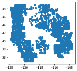
glas_gdf.plot();

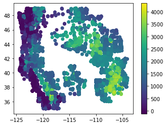
glas_gdf.plot(column='glas_z', legend=True)

<AxesSubplot:>

glas_gdf.total_bounds

array([-124.482406,   34.999455, -104.052336,   48.999727])

glas_gdf.geometry

0        POINT (-105.35656 44.15790)
1        POINT (-105.35812 44.15017)
2        POINT (-105.35843 44.14863)
3        POINT (-105.35874 44.14709)
4        POINT (-105.35905 44.14554)
                    ...             
65231    POINT (-117.04440 37.89622)
65232    POINT (-117.04467 37.89777)
65233    POINT (-117.04495 37.89932)
65234    POINT (-117.04523 37.90087)
65235    POINT (-117.04551 37.90242)
Name: geometry, Length: 65236, dtype: geometry

#glas_gdf.explore()

Reproject the GeoDataFrame

#glas_gdf.to_crs?

glas_gdf_proj = glas_gdf.to_crs('EPSG:3857')

glas_gdf_proj.head()

	decyear	ordinal	lat	lon	glas_z	dem_z	dem_z_std	lulc	geometry
0	2003.139571	731266.943345	44.157897	-105.356562	1398.51	1400.52	0.33	31	POINT (-11728238.834 5489909.710)
1	2003.139571	731266.943346	44.150175	-105.358116	1387.11	1384.64	0.43	31	POINT (-11728411.824 5488711.598)
2	2003.139571	731266.943347	44.148632	-105.358427	1392.83	1383.49	0.28	31	POINT (-11728446.444 5488472.212)
3	2003.139571	731266.943347	44.147087	-105.358738	1384.24	1382.85	0.84	31	POINT (-11728481.065 5488232.521)
4	2003.139571	731266.943347	44.145542	-105.359048	1369.21	1380.24	1.73	31	POINT (-11728515.574 5487992.837)

glas_gdf_proj.crs

<Derived Projected CRS: EPSG:3857>
Name: WGS 84 / Pseudo-Mercator
Axis Info [cartesian]:
- X[east]: Easting (metre)
- Y[north]: Northing (metre)
Area of Use:
- name: World between 85.06°S and 85.06°N.
- bounds: (-180.0, -85.06, 180.0, 85.06)
Coordinate Operation:
- name: Popular Visualisation Pseudo-Mercator
- method: Popular Visualisation Pseudo Mercator
Datum: World Geodetic System 1984 ensemble
- Ellipsoid: WGS 84
- Prime Meridian: Greenwich

#glas_gdf.plot();

#glas_gdf_proj.plot();

CRS and Projections

There are many excellent references out there about coordinate systems and map projections. I’m not going to try to reproduce here. If you’re relatively new to all of this, please revisit resources in the reading assignment. Can also review:

• https://www.axismaps.com/guide/map-projections

• http://downloads2.esri.com/support/documentation/ao_/710Understanding_Map_Projections.pdf

• https://courses.washington.edu/gis250/lessons/projection/

I particularly like this poster from the USGS: https://pubs.er.usgs.gov/publication/70047422

Coordinate Reference System (CRS)

• CRS is a “coordinate system with a datum”

• AKA Spatial Reference System (SRS): https://en.wikipedia.org/wiki/Spatial_reference_system

• Two types:

  • Geodetic (AKA Geographic)

  • Projected

• https://datacarpentry.org/organization-geospatial/03-crs/

How to specify a CRS

Many ways! https://geopandas.org/en/stable/docs/user_guide/projections.html

• EPSG Codes

• Proj strings

• WKT and WKT2

  • https://en.wikipedia.org/wiki/Well-known_text_representation_of_coordinate_reference_systems

!gdalsrsinfo EPSG:4326

PROJ.4 : +proj=longlat +datum=WGS84 +no_defs

OGC WKT2:2018 :
GEOGCRS["WGS 84",
    ENSEMBLE["World Geodetic System 1984 ensemble",
        MEMBER["World Geodetic System 1984 (Transit)"],
        MEMBER["World Geodetic System 1984 (G730)"],
        MEMBER["World Geodetic System 1984 (G873)"],
        MEMBER["World Geodetic System 1984 (G1150)"],
        MEMBER["World Geodetic System 1984 (G1674)"],
        MEMBER["World Geodetic System 1984 (G1762)"],
        MEMBER["World Geodetic System 1984 (G2139)"],
        ELLIPSOID["WGS 84",6378137,298.257223563,
            LENGTHUNIT["metre",1]],
        ENSEMBLEACCURACY[2.0]],
    PRIMEM["Greenwich",0,
        ANGLEUNIT["degree",0.0174532925199433]],
    CS[ellipsoidal,2],
        AXIS["geodetic latitude (Lat)",north,
            ORDER[1],
            ANGLEUNIT["degree",0.0174532925199433]],
        AXIS["geodetic longitude (Lon)",east,
            ORDER[2],
            ANGLEUNIT["degree",0.0174532925199433]],
    USAGE[
        SCOPE["Horizontal component of 3D system."],
        AREA["World."],
        BBOX[-90,-180,90,180]],
    ID["EPSG",4326]]

!gdalsrsinfo EPSG:32610

PROJ.4 : +proj=utm +zone=10 +datum=WGS84 +units=m +no_defs

OGC WKT2:2018 :
PROJCRS["WGS 84 / UTM zone 10N",
    BASEGEOGCRS["WGS 84",
        ENSEMBLE["World Geodetic System 1984 ensemble",
            MEMBER["World Geodetic System 1984 (Transit)"],
            MEMBER["World Geodetic System 1984 (G730)"],
            MEMBER["World Geodetic System 1984 (G873)"],
            MEMBER["World Geodetic System 1984 (G1150)"],
            MEMBER["World Geodetic System 1984 (G1674)"],
            MEMBER["World Geodetic System 1984 (G1762)"],
            MEMBER["World Geodetic System 1984 (G2139)"],
            ELLIPSOID["WGS 84",6378137,298.257223563,
                LENGTHUNIT["metre",1]],
            ENSEMBLEACCURACY[2.0]],
        PRIMEM["Greenwich",0,
            ANGLEUNIT["degree",0.0174532925199433]],
        ID["EPSG",4326]],
    CONVERSION["UTM zone 10N",
        METHOD["Transverse Mercator",
            ID["EPSG",9807]],
        PARAMETER["Latitude of natural origin",0,
            ANGLEUNIT["degree",0.0174532925199433],
            ID["EPSG",8801]],
        PARAMETER["Longitude of natural origin",-123,
            ANGLEUNIT["degree",0.0174532925199433],
            ID["EPSG",8802]],
        PARAMETER["Scale factor at natural origin",0.9996,
            SCALEUNIT["unity",1],
            ID["EPSG",8805]],
        PARAMETER["False easting",500000,
            LENGTHUNIT["metre",1],
            ID["EPSG",8806]],
        PARAMETER["False northing",0,
            LENGTHUNIT["metre",1],
            ID["EPSG",8807]]],
    CS[Cartesian,2],
        AXIS["(E)",east,
            ORDER[1],
            LENGTHUNIT["metre",1]],
        AXIS["(N)",north,
            ORDER[2],
            LENGTHUNIT["metre",1]],
    USAGE[
        SCOPE["Engineering survey, topographic mapping."],
        AREA["Between 126°W and 120°W, northern hemisphere between equator and 84°N, onshore and offshore. Canada - British Columbia (BC); Northwest Territories (NWT); Nunavut; Yukon. United States (USA) - Alaska (AK)."],
        BBOX[0,-126,84,-120]],
    ID["EPSG",32610]]

Map Projection check in

• https://en.wikipedia.org/wiki/Map_projection

• Tradeoffs - no perfect projection, all have some distortion of distance, area, direction, shape

• Infinite number of ways to represent the Earth’s 3D surface on a 2D Plane

  • Plane (azimuthal), Cone, Cylinder

  • Tangent, Secant (intersects sphere at two locations)

  • Different parameters for different definitions

    • Center longitude, center latitude

    • Lines of “true scale”

Proj strings

mycrs = glas_gdf.crs
mycrs

<Geographic 2D CRS: EPSG:4326>
Name: WGS 84
Axis Info [ellipsoidal]:
- Lat[north]: Geodetic latitude (degree)
- Lon[east]: Geodetic longitude (degree)
Area of Use:
- name: World.
- bounds: (-180.0, -90.0, 180.0, 90.0)
Datum: World Geodetic System 1984 ensemble
- Ellipsoid: WGS 84
- Prime Meridian: Greenwich

mycrs.to_epsg()

4326

mycrs.to_proj4()
#Note warning

/srv/conda/envs/notebook/lib/python3.9/site-packages/pyproj/crs/crs.py:1256: UserWarning: You will likely lose important projection information when converting to a PROJ string from another format. See: https://proj.org/faq.html#what-is-the-best-format-for-describing-coordinate-reference-systems
  return self._crs.to_proj4(version=version)

'+proj=longlat +datum=WGS84 +no_defs +type=crs'

glas_gdf_proj.crs.to_epsg()

3857

glas_gdf_proj.crs.to_proj4()

'+proj=merc +a=6378137 +b=6378137 +lat_ts=0 +lon_0=0 +x_0=0 +y_0=0 +k=1 +units=m +nadgrids=@null +wktext +no_defs +type=crs'

proj_str = '+proj=sinu'

glas_gdf.to_crs(proj_str)

	decyear	ordinal	lat	lon	glas_z	dem_z	dem_z_std	lulc	geometry
0	2003.139571	731266.943345	44.157897	-105.356562	1398.51	1400.52	0.33	31	POINT (-8427806.282 4891366.903)
1	2003.139571	731266.943346	44.150175	-105.358116	1387.11	1384.64	0.43	31	POINT (-8429029.663 4890508.871)
2	2003.139571	731266.943347	44.148632	-105.358427	1392.83	1383.49	0.28	31	POINT (-8429274.141 4890337.420)
3	2003.139571	731266.943347	44.147087	-105.358738	1384.24	1382.85	0.84	31	POINT (-8429518.899 4890165.747)
4	2003.139571	731266.943347	44.145542	-105.359048	1369.21	1380.24	1.73	31	POINT (-8429763.572 4889994.074)
...	...	...	...	...	...	...	...	...	...
65231	2009.775995	733691.238340	37.896222	-117.044399	1556.16	1556.43	0.00	31	POINT (-10294767.886 4195979.129)
65232	2009.775995	733691.238340	37.897769	-117.044675	1556.02	1556.43	0.00	31	POINT (-10294576.705 4196150.837)
65233	2009.775995	733691.238340	37.899319	-117.044952	1556.19	1556.44	0.00	31	POINT (-10294385.184 4196322.879)
65234	2009.775995	733691.238340	37.900869	-117.045230	1556.18	1556.44	0.00	31	POINT (-10294193.744 4196494.920)
65235	2009.775995	733691.238341	37.902420	-117.045508	1556.32	1556.44	0.00	31	POINT (-10294002.155 4196667.073)

65236 rows × 9 columns

Combining Vector Data

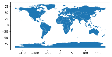
#Grab the bundled world polygons
world = gpd.read_file(gpd.datasets.get_path('naturalearth_lowres'))

world

	pop_est	continent	name	iso_a3	gdp_md_est	geometry
0	920938	Oceania	Fiji	FJI	8374.0	MULTIPOLYGON (((180.00000 -16.06713, 180.00000...
1	53950935	Africa	Tanzania	TZA	150600.0	POLYGON ((33.90371 -0.95000, 34.07262 -1.05982...
2	603253	Africa	W. Sahara	ESH	906.5	POLYGON ((-8.66559 27.65643, -8.66512 27.58948...
3	35623680	North America	Canada	CAN	1674000.0	MULTIPOLYGON (((-122.84000 49.00000, -122.9742...
4	326625791	North America	United States of America	USA	18560000.0	MULTIPOLYGON (((-122.84000 49.00000, -120.0000...
...	...	...	...	...	...	...
172	7111024	Europe	Serbia	SRB	101800.0	POLYGON ((18.82982 45.90887, 18.82984 45.90888...
173	642550	Europe	Montenegro	MNE	10610.0	POLYGON ((20.07070 42.58863, 19.80161 42.50009...
174	1895250	Europe	Kosovo	-99	18490.0	POLYGON ((20.59025 41.85541, 20.52295 42.21787...
175	1218208	North America	Trinidad and Tobago	TTO	43570.0	POLYGON ((-61.68000 10.76000, -61.10500 10.890...
176	13026129	Africa	S. Sudan	SSD	20880.0	POLYGON ((30.83385 3.50917, 29.95350 4.17370, ...

177 rows × 6 columns

world.crs

<Geographic 2D CRS: EPSG:4326>
Name: WGS 84
Axis Info [ellipsoidal]:
- Lat[north]: Geodetic latitude (degree)
- Lon[east]: Geodetic longitude (degree)
Area of Use:
- name: World.
- bounds: (-180.0, -90.0, 180.0, 90.0)
Datum: World Geodetic System 1984 ensemble
- Ellipsoid: WGS 84
- Prime Meridian: Greenwich

world.geometry

0      MULTIPOLYGON (((180.00000 -16.06713, 180.00000...
1      POLYGON ((33.90371 -0.95000, 34.07262 -1.05982...
2      POLYGON ((-8.66559 27.65643, -8.66512 27.58948...
3      MULTIPOLYGON (((-122.84000 49.00000, -122.9742...
4      MULTIPOLYGON (((-122.84000 49.00000, -120.0000...
                             ...                        
172    POLYGON ((18.82982 45.90887, 18.82984 45.90888...
173    POLYGON ((20.07070 42.58863, 19.80161 42.50009...
174    POLYGON ((20.59025 41.85541, 20.52295 42.21787...
175    POLYGON ((-61.68000 10.76000, -61.10500 10.890...
176    POLYGON ((30.83385 3.50917, 29.95350 4.17370, ...
Name: geometry, Length: 177, dtype: geometry

world.plot();

Select a country by name

idx = world['name'] == 'United States of America'

idx

0      False
1      False
2      False
3      False
4       True
       ...  
172    False
173    False
174    False
175    False
176    False
Name: name, Length: 177, dtype: bool

us = world[idx]
us

	pop_est	continent	name	iso_a3	gdp_md_est	geometry
4	326625791	North America	United States of America	USA	18560000.0	MULTIPOLYGON (((-122.84000 49.00000, -120.0000...

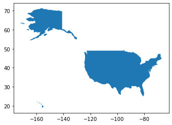
us.plot()

<AxesSubplot:>

us.crs

<Geographic 2D CRS: EPSG:4326>
Name: WGS 84
Axis Info [ellipsoidal]:
- Lat[north]: Geodetic latitude (degree)
- Lon[east]: Geodetic longitude (degree)
Area of Use:
- name: World.
- bounds: (-180.0, -90.0, 180.0, 90.0)
Datum: World Geodetic System 1984 ensemble
- Ellipsoid: WGS 84
- Prime Meridian: Greenwich

us.geometry

4    MULTIPOLYGON (((-122.84000 49.00000, -120.0000...
Name: geometry, dtype: geometry

Compute area

us.area
#Note warning!

/tmp/ipykernel_652/4249169899.py:1: UserWarning: Geometry is in a geographic CRS. Results from 'area' are likely incorrect. Use 'GeoSeries.to_crs()' to re-project geometries to a projected CRS before this operation.

  us.area

4    1122.281921
dtype: float64

Note: All calculations in GEOS/Shapely are simple euclidian geometry calculations in a 2D cartesian coordinate system!

Use an equal area projection!

• https://proj.org/operations/projections/cea.html

us_cea = us.to_crs('+proj=cea')
us_cea

	pop_est	continent	name	iso_a3	gdp_md_est	geometry
4	326625791	North America	United States of America	USA	18560000.0	MULTIPOLYGON (((-13674486.249 4793613.071, -13...

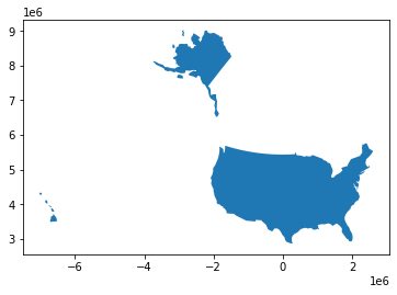
us_cea.plot()

<AxesSubplot:>

us_cea.area

4    9.509851e+12
dtype: float64

us_cea.area/1E6

4    9.509851e+06
dtype: float64

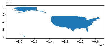
us_cea = us.to_crs('+proj=tmerc +lon_0=-100')
us_cea.plot()

<AxesSubplot:>

#Back to Web Mercator
#us_cea.explore()

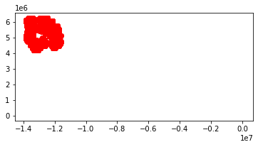
Combining on same plot

#%matplotlib widget

f, ax = plt.subplots()
us.plot(ax=ax)
glas_gdf_proj.plot(ax=ax, color='r');

#Where are the US polygons?  Let's take a look...

Use a common projection!

us_proj = us.to_crs(glas_gdf_proj.crs)
us_proj

	pop_est	continent	name	iso_a3	gdp_md_est	geometry
4	326625791	North America	United States of America	USA	18560000.0	MULTIPOLYGON (((-13674486.249 6274861.394, -13...

us_proj.crs

<Derived Projected CRS: EPSG:3857>
Name: WGS 84 / Pseudo-Mercator
Axis Info [cartesian]:
- X[east]: Easting (metre)
- Y[north]: Northing (metre)
Area of Use:
- name: World between 85.06°S and 85.06°N.
- bounds: (-180.0, -85.06, 180.0, 85.06)
Coordinate Operation:
- name: Popular Visualisation Pseudo-Mercator
- method: Popular Visualisation Pseudo Mercator
Datum: World Geodetic System 1984 ensemble
- Ellipsoid: WGS 84
- Prime Meridian: Greenwich

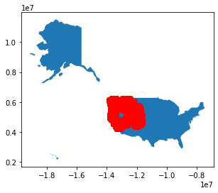
f, ax = plt.subplots()
us_proj.plot(ax=ax)
glas_gdf_proj.plot(ax=ax, color='r');

# Much better!