.ipynb .pdf

repository open issue

Binder

Contents

Excercises 2

Notebook #2: WA state hourly data

UW Geospatial Data Analysis
CEE498/CEWA599
David Shean

import os
from glob import glob
import numpy as np
import xarray as xr
import pandas as pd
import geopandas as gpd
import cartopy.crs as ccrs
import matplotlib.pyplot as plt

Part 2: Hourly data for WA state

Load the WA temperature, precipitation and snow depth products

• Note: these are extracted for 12:00 UTC

• Really want daily averages for much of this, but I didn’t have time to go back and requery ERA5

• Let’s use what we have to play around

#fn = 'WA_era5-land-monthly_averaged_reanalysis_by_hour_of_day.grib'
#wa_t = xr.open_dataset(fn, engine='cfgrib')

fn_list = ['era5_data/era5_WA_1979-2021_6hr/era5_WA_1979-2021_6hr_2m_temperature.nc', \
           'era5_data/era5_WA_1979-2021_6hr/era5_WA_1979-2021_6hr_total_precipitation.nc', 
           'era5_data/era5_WA_1979-2021_6hr/era5_WA_1979-2021_6hr_snow_depth.nc']

Use open_mfdataset to merge when opening

• Could have used open_dataset on each nc, then combined

• http://xarray.pydata.org/en/stable/generated/xarray.open_mfdataset.html

• See more details on merge/combine in xarray: http://xarray.pydata.org/en/stable/combining.html

#Specify chunks to split
#chunks={'time':2048}
chunks=None

wa_merge = xr.open_mfdataset(fn_list, combine='by_coords', chunks=chunks)
wa_merge = wa_merge.sel(step=0)

wa_merge

<xarray.Dataset>
Dimensions:    (latitude: 13, longitude: 30, time: 61592)
Coordinates:
  * time       (time) datetime64[ns] 1979-01-01 ... 2021-02-26T18:00:00
  * latitude   (latitude) float64 48.75 48.5 48.25 48.0 ... 46.25 46.0 45.75
  * longitude  (longitude) float64 -124.5 -124.2 -124.0 ... -117.8 -117.5 -117.2
Data variables:
    sd         (time, latitude, longitude) float32 dask.array<chunksize=(61592, 13, 30), meta=np.ndarray>
    t2m        (time, latitude, longitude) float32 dask.array<chunksize=(61592, 13, 30), meta=np.ndarray>
    tp         (time, latitude, longitude) float32 dask.array<chunksize=(61592, 13, 30), meta=np.ndarray>
Attributes:
    GRIB_edition:            1
    GRIB_centre:             ecmf
    GRIB_centreDescription:  European Centre for Medium-Range Weather Forecasts
    GRIB_subCentre:          0
    Conventions:             CF-1.7
    institution:             European Centre for Medium-Range Weather Forecasts
    history:                 2021-03-04T16:33:29 GRIB to CDM+CF via cfgrib-0....

wa_merge['t2m'] -= 273.15
wa_merge['t2m'].attrs['units'] = 'C'

#Convert meters to mm
wa_merge['tp'] *= 1000
wa_merge['tp'].attrs['units'] = 'mm'

wa_merge['t2m']

<xarray.DataArray 't2m' (time: 61592, latitude: 13, longitude: 30)>
dask.array<sub, shape=(61592, 13, 30), dtype=float32, chunksize=(61592, 13, 30), chunktype=numpy.ndarray>
Coordinates:
  * time       (time) datetime64[ns] 1979-01-01 ... 2021-02-26T18:00:00
  * latitude   (latitude) float64 48.75 48.5 48.25 48.0 ... 46.25 46.0 45.75
  * longitude  (longitude) float64 -124.5 -124.2 -124.0 ... -117.8 -117.5 -117.2
Attributes:
    GRIB_paramId:                             167
    GRIB_shortName:                           2t
    GRIB_units:                               K
    GRIB_name:                                2 metre temperature
    GRIB_cfVarName:                           t2m
    GRIB_dataType:                            an
    GRIB_missingValue:                        9999
    GRIB_numberOfPoints:                      390
    GRIB_totalNumber:                         0
    GRIB_typeOfLevel:                         surface
    GRIB_NV:                                  0
    GRIB_stepUnits:                           1
    GRIB_stepType:                            instant
    GRIB_gridType:                            regular_ll
    GRIB_gridDefinitionDescription:           Latitude/Longitude Grid
    GRIB_Nx:                                  30
    GRIB_iDirectionIncrementInDegrees:        0.25
    GRIB_iScansNegatively:                    0
    GRIB_longitudeOfFirstGridPointInDegrees:  -124.5
    GRIB_longitudeOfLastGridPointInDegrees:   -117.25
    GRIB_Ny:                                  13
    GRIB_jDirectionIncrementInDegrees:        0.25
    GRIB_jPointsAreConsecutive:               0
    GRIB_jScansPositively:                    0
    GRIB_latitudeOfFirstGridPointInDegrees:   48.75
    GRIB_latitudeOfLastGridPointInDegrees:    45.75
    long_name:                                2 metre temperature
    units:                                    C
    coordinates:                              number time step surface latitu...

#wa_merge = wa_merge.dropna(dim='time')

#Unset units (avoid plotting in x and y label)
wa_merge['latitude'].attrs['units'] = None
wa_merge['longitude'].attrs['units'] = None

Clip to WA state geometry

#wa_merge_clip = wa_merge.rio.write_crs(world.crs);
#wa_merge_clip = wa_merge_clip.rio.clip(wa_geom, crs=world.crs, drop=False)

Compute seasonal mean values for each variable

• This is a simple groupby() and mean()

• Inspect the output values - do these make sense?

wa_merge_seasonal_mean = wa_merge.groupby('time.season').mean()

wa_merge_seasonal_mean

<xarray.Dataset>
Dimensions:    (latitude: 13, longitude: 30, season: 4)
Coordinates:
  * latitude   (latitude) float64 48.75 48.5 48.25 48.0 ... 46.25 46.0 45.75
  * longitude  (longitude) float64 -124.5 -124.2 -124.0 ... -117.8 -117.5 -117.2
  * season     (season) object 'DJF' 'JJA' 'MAM' 'SON'
Data variables:
    sd         (season, latitude, longitude) float32 dask.array<chunksize=(1, 13, 30), meta=np.ndarray>
    t2m        (season, latitude, longitude) float32 dask.array<chunksize=(1, 13, 30), meta=np.ndarray>
    tp         (season, latitude, longitude) float32 dask.array<chunksize=(1, 13, 30), meta=np.ndarray>

#Hack to reorder seasons, as default is alphabetical
#order = np.array(['DJF', 'MAM', 'JJA', 'SON'], dtype=object)
order = np.array([0,2,1,3])
#wa_merge_seasonal_mean.season.values
wa_merge_seasonal_mean = wa_merge_seasonal_mean.isel(season=order)

#wa_merge_seasonal_resample = wa_merge.resample(time='Q-NOV').mean('time')

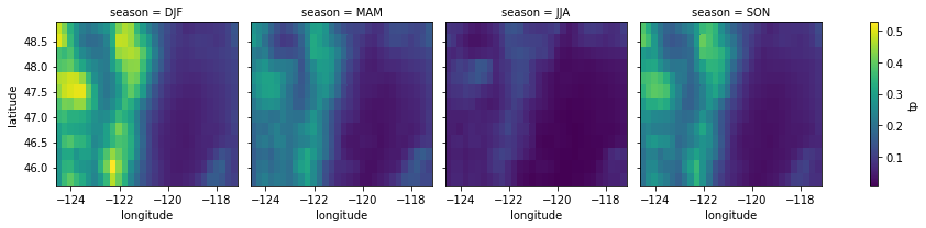
Plot seasonal mean grids

• Note that plot will assume x='longitude', y='latitude', but can also explicitly specify

wa_merge_seasonal_mean.data_vars

Data variables:
    sd       (season, latitude, longitude) float32 dask.array<chunksize=(1, 13, 30), meta=np.ndarray>
    t2m      (season, latitude, longitude) float32 dask.array<chunksize=(1, 13, 30), meta=np.ndarray>
    tp       (season, latitude, longitude) float32 dask.array<chunksize=(1, 13, 30), meta=np.ndarray>

for i in wa_merge_seasonal_mean.data_vars:
    wa_merge_seasonal_mean[i].plot(col='season')

Compute mean monthly values for WA state

wa_monthly_mean = wa_merge.groupby('time.month').mean('time').mean(['latitude','longitude'])
wa_monthly_mean

<xarray.Dataset>
Dimensions:  (month: 12)
Coordinates:
  * month    (month) int64 1 2 3 4 5 6 7 8 9 10 11 12
Data variables:
    sd       (month) float32 dask.array<chunksize=(1,), meta=np.ndarray>
    t2m      (month) float32 dask.array<chunksize=(1,), meta=np.ndarray>
    tp       (month) float32 dask.array<chunksize=(1,), meta=np.ndarray>

f, axa = plt.subplots(3,1, sharex=True)
wa_monthly_mean['t2m'].plot(ax=axa[0])
wa_monthly_mean['tp'].plot(ax=axa[1])
wa_monthly_mean['sd'].plot(ax=axa[2]);

Helper function for plotting WA grids with state outline overlay

def plotwa(ds_in, v_list=['t2m','tp','sd'], op='mean'):
    f,axa = plt.subplots(1,3, figsize=(12,2), sharex=True, sharey=True)
    for i,v in enumerate(v_list):
        ds_in[v].plot(ax=axa[i], robust=True)
        wa_state.plot(ax=axa[i], facecolor='none', edgecolor='black')
        axa[i].set_title('WA State ERA5 Hourly: %s %s' % (op, v))
    f.tight_layout()

Get the WA state outline

#states_url = 'http://eric.clst.org/assets/wiki/uploads/Stuff/gz_2010_us_040_00_5m.json'
states_url = 'http://eric.clst.org/assets/wiki/uploads/Stuff/gz_2010_us_040_00_500k.json'
states_gdf = gpd.read_file(states_url)

wa_state = states_gdf.loc[states_gdf['NAME'] == 'Washington']

wa_state.plot();

wa_geom = wa_state.iloc[0].geometry
wa_geom

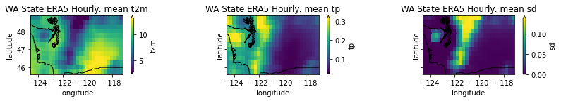
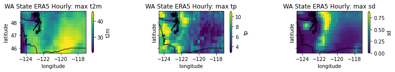
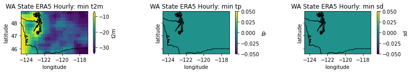
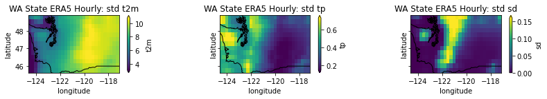
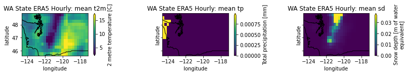
Create some plots of descriptive stats (mean, max, min, std) for 1979-present

• Pass the relevant dataset (e.g. wa_merge.mean('time')) to the plotwa helper function

• What do these metrics tell you?

  • What is causing most of the temperature variability captured by the std?

  • What is the highest temperature value

plotwa(wa_merge.mean('time'), op='mean')

plotwa(wa_merge.max('time'), op='max')

plotwa(wa_merge.min('time'), op='min')

plotwa(wa_merge.std('time'), op='std')

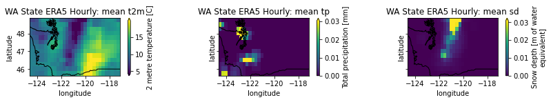
Create a plot showing the conditions the day before and after the Mt. St. Helen’s eruption

pre = wa_merge.sel(time='1980-05-18T06:00')
plotwa(pre)
post = wa_merge.sel(time='1980-05-19T06:00')
plotwa(post)

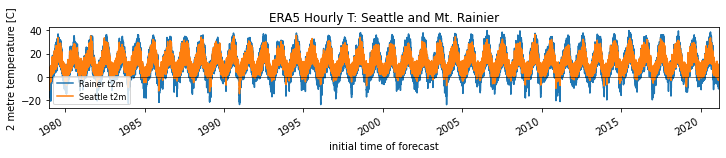
Extract the time series for Seattle and Mt. Rainier temperature and create line plot

• You’ll need to look up coordinates

  • Check the longitude system in the DataArrays (-180 to 180, or 0 to 360)

• Can use the sel() method to extract time series for the grid cell nearest the specified ‘longitude’ and ‘latitude’ coordinates

  • http://xarray.pydata.org/en/stable/indexing.html

  • Remember, these are large grid cells (~31x31 km), so one grid cell could cover the most of Mt. Rainier (a single temperature value that includes the cold summit and the warmer, lowland river valleys)

• Sanity check

sea_coord = (-122.25, 47.5)
rainier_coord = (121.7603, 46.8523)

sea_ts = wa_merge.sel(longitude=sea_coord[0], latitude=sea_coord[1], method='nearest')
sea_ts

<xarray.Dataset>
Dimensions:    (time: 61592)
Coordinates:
  * time       (time) datetime64[ns] 1979-01-01 ... 2021-02-26T18:00:00
    latitude   float64 47.5
    longitude  float64 -122.2
Data variables:
    sd         (time) float32 dask.array<chunksize=(61592,), meta=np.ndarray>
    t2m        (time) float32 dask.array<chunksize=(61592,), meta=np.ndarray>
    tp         (time) float32 dask.array<chunksize=(61592,), meta=np.ndarray>
Attributes:
    GRIB_edition:            1
    GRIB_centre:             ecmf
    GRIB_centreDescription:  European Centre for Medium-Range Weather Forecasts
    GRIB_subCentre:          0
    Conventions:             CF-1.7
    institution:             European Centre for Medium-Range Weather Forecasts
    history:                 2021-03-04T16:33:29 GRIB to CDM+CF via cfgrib-0....

rainier_ts = wa_merge.sel(longitude=rainier_coord[0], latitude=rainier_coord[1], method='nearest')
rainier_ts

<xarray.Dataset>
Dimensions:    (time: 61592)
Coordinates:
  * time       (time) datetime64[ns] 1979-01-01 ... 2021-02-26T18:00:00
    latitude   float64 46.75
    longitude  float64 -117.2
Data variables:
    sd         (time) float32 dask.array<chunksize=(61592,), meta=np.ndarray>
    t2m        (time) float32 dask.array<chunksize=(61592,), meta=np.ndarray>
    tp         (time) float32 dask.array<chunksize=(61592,), meta=np.ndarray>
Attributes:
    GRIB_edition:            1
    GRIB_centre:             ecmf
    GRIB_centreDescription:  European Centre for Medium-Range Weather Forecasts
    GRIB_subCentre:          0
    Conventions:             CF-1.7
    institution:             European Centre for Medium-Range Weather Forecasts
    history:                 2021-03-04T16:33:29 GRIB to CDM+CF via cfgrib-0....

rainier_ts.time.values.min()

numpy.datetime64('1979-01-01T00:00:00.000000000')

f, ax = plt.subplots(figsize=(12,1.5))
v = 't2m'
rainier_ts[v].plot(ax=ax, label='Rainer %s' % v)
sea_ts[v].plot(ax=ax, label='Seattle %s' % v)
ax.axhline(0,color='k',lw=0.5)
ax.legend(fontsize=8)
ax.set_xlim(rainier_ts.time.values.min(), rainier_ts.time.values.max())
ax.set_title("ERA5 Hourly T: Seattle and Mt. Rainier");

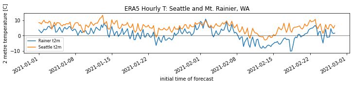
f, ax = plt.subplots(figsize=(12,1.5))
v = 't2m'
cy = 2021
rainier_ts[v].loc[f'{cy}-01-01':].plot(ax=ax, label='Rainer %s' % v)
sea_ts[v].loc[f'{cy}-01-01':].plot(ax=ax, label='Seattle %s' % v)
ax.axhline(0,color='k',lw=0.5)
ax.legend(fontsize=8)
ax.set_title("ERA5 Hourly T: Seattle and Mt. Rainier, WA");

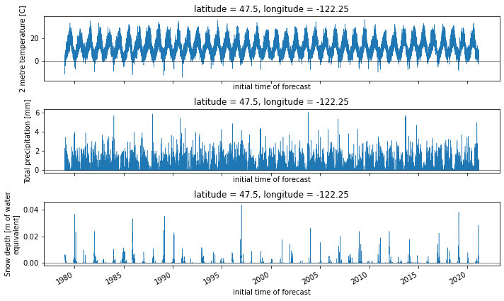
Helper function to plot time series

def plotv(ds_in, v_list=['t2m','tp','sd']):
    f,axa = plt.subplots(3,1, figsize=(10,6), sharex=True)
    for i,v in enumerate(v_list):
        ds_in[v].dropna(dim='time').plot(ax=axa[i], lw=0.5)
        axa[i].axhline(0,color='k',lw=0.5)
    f.tight_layout()

plotv(wa_merge.sel(longitude=sea_coord[0], latitude=sea_coord[1], method='nearest'))

plotv(wa_merge.sel(longitude=rainier_coord[0], latitude=rainier_coord[1], method='nearest'))

Compute stats for monthly, annual time periods

• Can use groupby('time.year').max(dim='time')

• Plot snow depth for April and September

Create a map that shows the year containing the maximum T value at each grid cell

• These should mostly be in the most recent decade

• Note the .compute() is needed to converty dask array to ndarray for use in vectorized indexing

max_t_idx = wa_merge['t2m'].argmax(dim='time').compute()

wa_merge['t2m']['time.year']

<xarray.DataArray 'year' (time: 61592)>
array([1979, 1979, 1979, ..., 2021, 2021, 2021])
Coordinates:
  * time     (time) datetime64[ns] 1979-01-01 ... 2021-02-26T18:00:00

f, ax = plt.subplots()
wa_merge['t2m']['time.year'][max_t_idx].plot(ax=ax)
wa_state.plot(ax=ax, facecolor='none', edgecolor='black');

wa_merge['t2m']['time.year'][max_t_idx].median()

<xarray.DataArray 'year' ()>
array(2006.)

Extra Credit

Create a new xarray Dataset with the SNOTEL data from Lab08

Export one of the derived WA grids to rasterio

• https://github.com/robintw/XArrayAndRasterio/blob/master/rasterio_to_xarray.py

Load SRTM DEM for WA

• Resample

Plot contours from SRTM DEM over temperature grid

Compute correlation between temperature and elevation

• https://github.com/pydata/xarray/issues/1115

Compute atmospheric temperature lapse rate using SRTM elevations

What if my data are too big?

• http://xarray.pydata.org/en/stable/dask.html

previous

Excercises 1

next

10: Conda, Dask, rioxarray