07 Raster2 Exercises

Reprojection, Clipping, Sampling, Zonal Stats

UW Geospatial Data Analysis
CEE467/CEWA567
David Shean

⚠️ Suggestion - shut down other unneeded kernels before running

import os
import requests
import numpy as np
import pandas as pd
import geopandas as gpd
import rasterio as rio
from rasterio import plot, mask
from rasterio.warp import calculate_default_transform, reproject, Resampling
import matplotlib.pyplot as plt
import rasterstats
import rioxarray
from matplotlib_scalebar.scalebar import ScaleBar

#%matplotlib widget

Part 0: Prepare DEM data

• Run the Jupyterbook demo notebook to query and download data (07_Raster2_DEMs_Warp_Clip_Sample_demo.ipynb)

• Update the dem_data path to the corresponding subdirectory in the jupyterbook repo

dem_data = '/home/jovyan/jupyterbook/book/modules/07_Raster2_DEMs_Warp_Clip_Sample/dem_data'

#We will use the Washington state 3-arcsec SRTM dataset for these exercises
dem_fn = os.path.join(dem_data, "WA_SRTMGL3.tif")
#dem_fn = os.path.join(dem_data, "WA_COP90.tif")

Reproject the WA DEM data using gdalwarp or rasterio

• See demo

• Output should be LZW compressed and Tiled

#Define desired CRS for output
dst_crs = 'EPSG:32610'

#Student Exercise

Open as rasterio dataset

• Store as src_proj variable

• Check profile and CRS to make sure things look good

#Student Exercise

Create a shaded relief map for the projected DEM

• See demo

#Student Exercise

Load as masked array with rasterio

#Student Exercise

hs_extent = rio.plot.plotting_extent(hs_src)

Load the states GeoDataFrame

#states_url = 'http://eric.clst.org/assets/wiki/uploads/Stuff/gz_2010_us_040_00_5m.json'
states_url = 'http://eric.clst.org/assets/wiki/uploads/Stuff/gz_2010_us_040_00_500k.json'
states_gdf = gpd.read_file(states_url)
#Reproject to match raster
states_gdf_proj = states_gdf.to_crs(src_proj.crs)
#Isolate WA state
wa_state = states_gdf_proj.loc[states_gdf_proj['NAME'] == 'Washington']
#Extract geometry to use for clipping
wa_geom = wa_state.iloc[0].geometry

Clip to WA state

• See demo

• Store output array and transform from rio.mask.mask as wa_ma and wa_ma_transform

• https://rasterio.readthedocs.io/en/latest/api/rasterio.mask.html

#Pass this in to the `rio.mask.mask` call (see demo)
rio_mask_kwargs = {'filled':False, 'crop':True, 'indexes':1}

#Student Exercise

• Determine the clipped extent for imshow in the projected CRS using the rio.plot.plotting_extent

#Student Exercise

(371115.31896165153, 971151.8939989337, 5043526.21288473, 5444604.739324637)

Part 1: DEM Visualization and Analysis

Create a color shaded relief map

• You should already have the projected, clipped DEM and the hillshade (from unclipped, projected DEM) loaded as arrays

• Create a plot overlaying color elevation values on the hillshade

  • It’s important to correctly set the extent for each of the two arrays when passing to imshow, otherwise they won’t line up correctly. We did this in Lab05.

  • Use imshow alpha to set transparency of the DEM

  • Add a colorbar

#Student Exercise

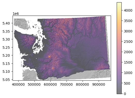
What is the maximum elevation in WA state

• According to your clipped DEM, not google :)

#Student Exercise

Extra Credit: What percentage of the state is >1 mile above sea level?

• Sorry about the imperial units, but this is what matters to your average hiking enthusiast

• Think back to Lab05 and the NDSI threshold appraoch to determine snow-covered area

• Remember, that you have a regular grid here, so you know the dimensions in meters of each grid cell

• As we know, this kind of calculation should be done in an equal-area projection, but fine to estimate with UTM projection here

#Student Exercise

#Student Exercise

#Student Exercise

Part 2: Volume estimation

• In the Raster 1 lab, we computed snow-covered area from a 2D array with known pixel dimensions (30x30 m for Landsat-8)

• Now, let’s add a third dimension to compute volume from a 2D array of elevation values

  • Imagine dividing the domain up into 1 cubic meter blocks - your elevation values are like stacks of these 1-m cubes above some reference datum

• Volume (and volume change) calculations are common operations with gridded DEMs. The analysis is often referred to as “cut/fill”. For example:

  • Measuring quarry slag pile volume

  • Measuring ice sheet and glacier change

• Let’s start with a simple example

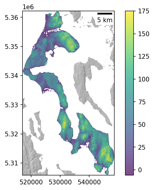
Compute the volume of Whidbey Island above sea level

• First, we need an area over which to compute volume

• Extract the Whidbey Island polygon from the WA state geometry

#If using the 500k state outlines, Whidbey is at index 7 in the MultiPolygon
whidbey_geom = wa_geom.geoms[7]
whidbey_geom

#Define a GeoSeries for easy plotting using GeoPandas
whidbey_gdf = gpd.GeoSeries(whidbey_geom)
whidbey_gdf

0    POLYGON ((535640.328 5348457.490, 535403.340 5...
dtype: geometry

• Now, mask the projected DEM dataset using this geometry

  • Note, rio.mask.mask expects an iterable “shape”, not a single geometry, so need to create and pass a single-element list object containing the whidbey_geom (something like [whidbey_geom,])

  • Use the same parameters that we used when clipping to the WA state geometry above

whidbey_ma, whidbey_out_transform = rio.mask.mask(src_proj, [whidbey_geom,], **rio_mask_kwargs)
whidbey_ma_extent = rio.plot.plotting_extent(whidbey_ma, whidbey_out_transform)

whidbey_ma_extent

(517068.30347175116, 548623.8474614524, 5305801.594847063, 5362175.333565047)

Create a plot of clipped Whidbey DEM

• Verify that you have a masked array of elevation values, with unmasked values only over the Whidbey polygon

• Extra credit: add hillshade, colorbar and scalebar

#Student Exercise

Define a “bottom” surface for our volume calculation

• Let’s use a constant elevation above the geoid (mean sea level) as our “baseline” elevation

  • Since our DEM values are height above the EGM96 geoid, we can use 0 here

  • Note that this bottom surface can also be more complex: a planar fit to elevations around a polygon, lake bathymetry, etc.

#Student Exercise

Compute the volume

• Compute the height of the DEM above this “baseline” elevation

• Convert the total volume to km^3

• Two potential methods:

  1. Use the known pixel size (remember res attribute of projected rasterio dataset) to compute the area of each pixel in m^2, then multiply by the height in m

  2. Determine mean height above the “baseline” elevation and multiply by total polygon area

• Try to do a sanity check here

#Student Exercise

#Student Exercise

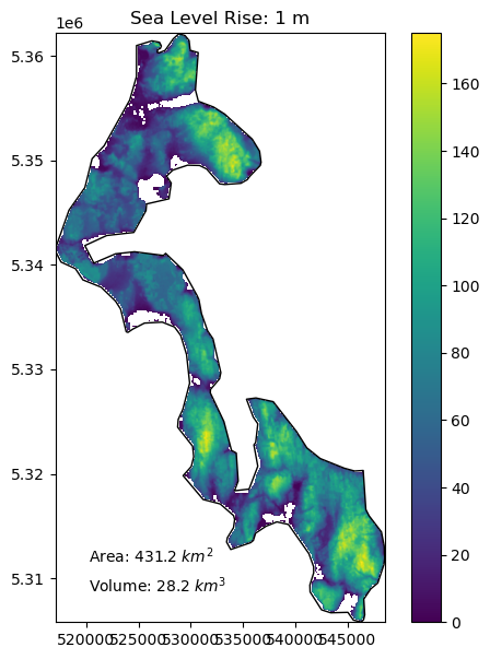
Volume estimate, method 1: 28.61 km3
Volume estimate, method 2: 29.47 km3

Note: The volume estimates from the two approaches are slightly different because the 500K polygon geometry is not quite the same as the mask that the DEM creators used to mask water. You can see this in the figure above, note areas with hillshade pixels but no color overlay.

We’re gonna need a bigger boat…

• Sea level rise is very real

  • Current global average rates are ~3.6 mm/yr

  • This may not sound like much, but over 100 years, thats 36 cm or ~1.2 feet! And the rate is increasing nonlinearly.

  • Some good references:

    • U.S. Interagency report from 2022: https://oceanservice.noaa.gov/hazards/sealevelrise/sealevelrise-tech-report.html

    • https://www.ipcc.ch/srocc/chapter/chapter-4-sea-level-rise-and-implications-for-low-lying-islands-coasts-and-communities/

    • https://archive.ipcc.ch/publications_and_data/ar4/wg1/en/faq-5-1.html

    • https://www.ipcc.ch/site/assets/uploads/2018/02/WG1AR5_Chapter13_FINAL.pdf

    • http://www.antarcticglaciers.org/glaciers-and-climate/what-is-the-global-volume-of-land-ice-and-how-is-it-changing/

• Let’s do some rough inundation calculations using our DEM

  • Note that in practice, we wouldn’t use a global DEM product like SRTM or COP30 for this, but would use a very accurate airborne lidar datset (like the most recent lidar data available from USGS 3DEP or WA DNR)

  • There are many other caveats here, as sea level rise is much more complex than just “filling the bathtub” (see the IPCC report), but we’re learning concepts and techniques, so let’s start with a simple case.

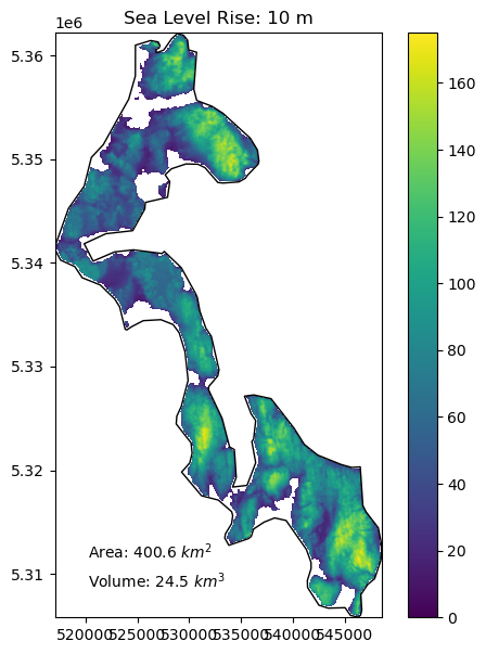
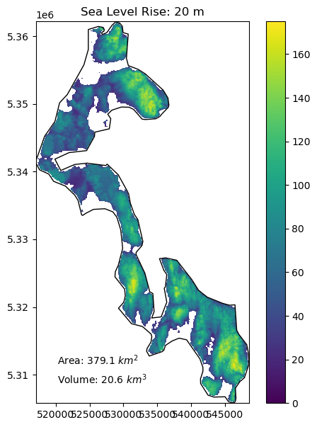
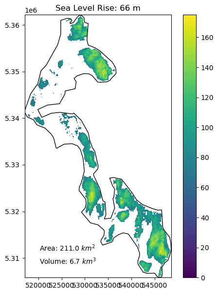
Create a function to compute the area and volume of whidbey island above sea level for:

• 1 meter of sea level rise

• 10 meters of sea level rise

• 20 meters of sea level rise

• 66 meters of sea level rise (roughly the total if all land ice melted, without accounting for thermal expansion)

Add a visualization component to your function

• Create plots using the whidbey Polygon as “reference shoreline”, and plot valid DEM values above the sea level with fixed color ramp limits

• Extra credit: add notation for area and volume above sea level

#def slr_plot(dem_ma, sl=0):

#Student Exercise

slr_values = (1,10,20,66)
for i in slr_values:
    slr_plot(whidbey_ma, sl=i)

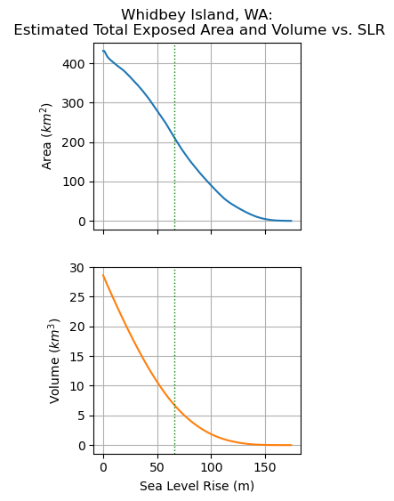
Extra Credit: Create area and volume inundation curves

• Starting with sea level of 0, increase by 1 m increments until Whidbey is totally submerged

• Create plots for:

  • exposed area vs sea level

  • exposed volume vs sea level

• Are the curves linear?

#Student Exercise

#Student Exercise

Part 3: Sampling a raster at points

Say you have some point data (e.g., lat/lon of field sites) and you need elevation values for your anlysis. Do you need to go back out and collect new GPS positions? No! You can extract elevation values from an existing DEM!

This is a surprisingly common requirement, though it is not always simple to implement. Let’s discuss a few options:

1. Simple rasterio sampling with integer indices using value from nearest raster cell (nearest neighbor)

2. Interpolated elevation from nearby pixels (e.g., bilinear interpolation)

3. Statistics extracted for a circular buffer around each point location (e.g., median for all pixels within 90 m radius of the point)

Sample the clipped WA DEM at the WA GLAS points

• Let’s start simple, using the rasterio sample function, which takes a list of (x,y) tuples in projected coordinates and returns nearest neighbor values from the raster

Load the GLAS points, reproject and clip to WA state

• We did all of this in previous labs, so I’m including sample code here

#Define path to the GLAS csv file
glas_fn = '~/jupyterbook/book/modules/01_Shell_Github/data/GLAH14_tllz_conus_lulcfilt_demfilt.csv'

#Prepare geodataframe
glas_df = pd.read_csv(glas_fn)
glas_gdf = gpd.GeoDataFrame(glas_df, crs='EPSG:4326', geometry=gpd.points_from_xy(glas_df['lon'], glas_df['lat']))

#Reproject to match our raster crs
glas_gdf_utm = glas_gdf.to_crs(src_proj.crs)

#Return points that intersect WA state geometry
glas_gdf_utm_wa = glas_gdf_utm.loc[glas_gdf_utm.intersects(wa_geom)]
glas_gdf_utm_wa.head()

	decyear	ordinal	lat	lon	glas_z	dem_z	dem_z_std	lulc	geometry
467	2003.143756	731268.470838	46.291775	-124.037745	-23.44	-23.53	0.00	31	POINT (420068.610 5126989.811)
468	2003.143756	731268.470838	46.293329	-124.038072	-23.11	-23.54	0.00	31	POINT (420045.685 5127162.809)
469	2003.143756	731268.470838	46.294880	-124.038399	-23.98	-22.78	0.26	31	POINT (420022.757 5127335.473)
470	2003.143756	731268.470840	46.302568	-124.040034	-24.61	-23.72	0.11	31	POINT (419908.041 5128191.352)
471	2003.143756	731268.470840	46.304107	-124.040358	-23.92	-23.73	0.00	31	POINT (419885.336 5128362.681)

Prepare the coordinate arrays to pass to rio sample function

• We touched on this in 05 demo and Lab05 when exploring the geotransform, corner coordinates and extracting values from the NumPy array. Maybe consult the demo, your code and/or the solutions.

  • https://uwgda-jupyterbook.readthedocs.io/en/latest/modules/05_Raster1_GDAL_rasterio_LS8/05_Raster1_GDAL_rasterio_demo.html#raster-and-array-sampling

  • The GeoPandas doc also has a simple example: https://geopandas.org/en/stable/gallery/geopandas_rasterio_sample.html

• The sample function expects a list of (x,y) tuples: https://rasterio.readthedocs.io/en/latest/api/rasterio.sample.html

  • Need to create this list of tuples from the Point geometry objects in your GeoDataFrame

  • Hint: Use list comprehension!

  • You want a list of the form [(x1,y1),(x2,y2),…]

• Pass to sample

• Note that the sample function returns a generator object, and it doesn’t actually evaluate the call!

• Can wrap the returned generator object in a np.array(list()) to evaluate, or use np.fromiter()

• This operation may take ~10-20 seconds to complete

I included some sample output for the first 10 records to make sure you’re on the right track.

#Student Exercise

First 10 records...

[(420068.6096560212, 5126989.811026542),
 (420045.6845556927, 5127162.808572696),
 (420022.756572206, 5127335.47293138),
 (419908.0411685074, 5128191.352440438),
 (419885.33555505634, 5128362.681306876),
 (410564.59385410615, 5197909.486655028),
 (410541.06220828043, 5198082.008111783),
 (410517.52547154634, 5198254.085230813),
 (401004.50357059937, 5269865.468511085),
 (400982.6047505999, 5270037.926469663)]

len(glas_coord)

5298

#Student Exercise

#Student Exercise

First 10 records...

array([  0,   0,   0,   0,   1,   0,   0,   4,  91, 132], dtype=int16)

Deal with nodata

• Some of our GLAS points are located over areas where we don’t have valid elevation measurements in the DEM

• These will have the raster nodata value (e.g., 0 in the SRTM-GL1 products)

• Set these to np.nan

#Check raster dataset nodata value
src_proj.nodata

0.0

#Need to convert to float here, as DEM samples are int16 and np.nan is float
glas_dem_elev = glas_dem_elev.astype(float)
glas_dem_elev[glas_dem_elev == src_proj.nodata] = np.nan
#glas_dem_elev = np.ma.masked_equal(glas_dem_elev, src_proj.nodata)

Store the sampled elevation values as a new column in the glas_gdf_utm_wa GeoDataFrame

glas_gdf_utm_wa['dem_rio_sample'] = glas_dem_elev
glas_gdf_utm_wa.head()

/srv/conda/envs/notebook/lib/python3.10/site-packages/geopandas/geodataframe.py:1443: SettingWithCopyWarning: 
A value is trying to be set on a copy of a slice from a DataFrame.
Try using .loc[row_indexer,col_indexer] = value instead

See the caveats in the documentation: https://pandas.pydata.org/pandas-docs/stable/user_guide/indexing.html#returning-a-view-versus-a-copy
  super().__setitem__(key, value)

	decyear	ordinal	lat	lon	glas_z	dem_z	dem_z_std	lulc	geometry	dem_rio_sample
467	2003.143756	731268.470838	46.291775	-124.037745	-23.44	-23.53	0.00	31	POINT (420068.610 5126989.811)	NaN
468	2003.143756	731268.470838	46.293329	-124.038072	-23.11	-23.54	0.00	31	POINT (420045.685 5127162.809)	NaN
469	2003.143756	731268.470838	46.294880	-124.038399	-23.98	-22.78	0.26	31	POINT (420022.757 5127335.473)	NaN
470	2003.143756	731268.470840	46.302568	-124.040034	-24.61	-23.72	0.11	31	POINT (419908.041 5128191.352)	NaN
471	2003.143756	731268.470840	46.304107	-124.040358	-23.92	-23.73	0.00	31	POINT (419885.336 5128362.681)	1.0

Create a plot of your new sampled elevation values

• Can visualize over shaded relief map or DEM

• Optional: include a subplot with GLAS values with same color scale

#Student Exercise

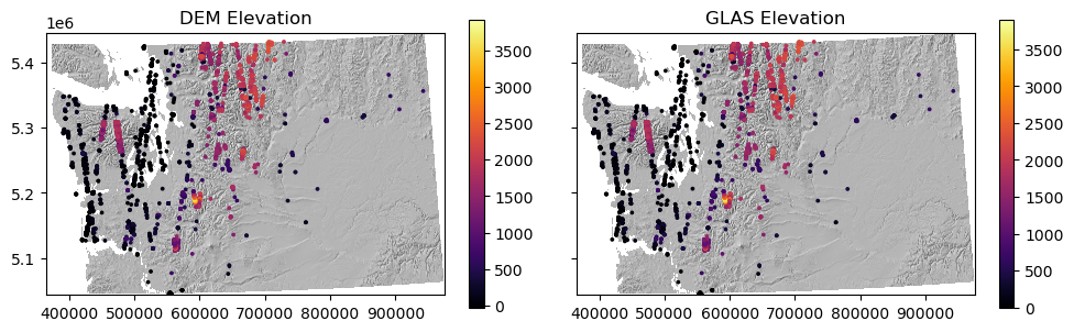
Extra Credit: Compare sampled DEM elevation with the GLAS elevation (glas_z)

glas_gdf_utm_wa['glas_dem_diff'] = glas_gdf_utm_wa['glas_z'] - glas_gdf_utm_wa['dem_rio_sample']

/srv/conda/envs/notebook/lib/python3.10/site-packages/geopandas/geodataframe.py:1443: SettingWithCopyWarning: 
A value is trying to be set on a copy of a slice from a DataFrame.
Try using .loc[row_indexer,col_indexer] = value instead

See the caveats in the documentation: https://pandas.pydata.org/pandas-docs/stable/user_guide/indexing.html#returning-a-view-versus-a-copy
  super().__setitem__(key, value)

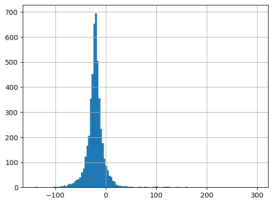
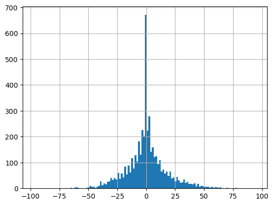
What is median offset?

• Think back to Lab03 where we learned about datums and elevations reported as height above ellipsoid vs. height above geoid (mean sea level)

glas_gdf_utm_wa['glas_dem_diff'].median()

-20.700000000000045

glas_gdf_utm_wa['glas_dem_diff'].hist(bins=128);

Prepare EGM96 geoid offset grid

#From PROJ7 cloud-hosted datum grids: https://cdn.proj.org/
url = 'https://cdn.proj.org/us_nga_egm96_15.tif'

src_egm96 = rio.open(url)
src_egm96.profile

{'driver': 'GTiff', 'dtype': 'float32', 'nodata': None, 'width': 1440, 'height': 721, 'count': 1, 'crs': CRS.from_epsg(4979), 'transform': Affine(0.25, 0.0, -180.125,
       0.0, -0.25, 90.125), 'blockxsize': 256, 'blockysize': 256, 'tiled': True, 'compress': 'deflate', 'interleave': 'band'}

egm96 = src_egm96.read(1)
egm96_extent = rio.plot.plotting_extent(src_egm96)
np.percentile(egm96, (2,98))

array([-60.25124443,  59.33671082])

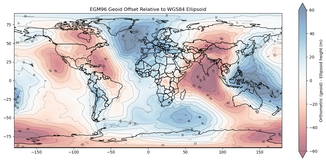
Prepare EGM96 offset grid figure

world = gpd.read_file(gpd.datasets.get_path('naturalearth_lowres'))

clim = (-60,60)
#Contour interval
cint = 10
clevels=np.arange(np.floor(egm96.min()/cint)*cint, np.ceil(egm96.max()/cint)*cint, cint)

#This function is defined later in the notebook
#egm96_hs,_,_ = hillshade(egm96)

f, ax = plt.subplots(figsize=(15,7))
m = ax.imshow(egm96, extent=egm96_extent, cmap='RdBu', clim=clim, alpha=0.5, zorder=1)
#ax.imshow(egm96_hs, cmap='gray', extent=egm96_extent, zorder=0)
ax.autoscale(False)
c_color = 'k'
cs = ax.contour(egm96, origin='image', extent=egm96_extent, linewidths=0.25, alpha=1.0, colors=c_color, levels=clevels)
ax.clabel(cs, inline=1, fmt='%0.0f', colors=c_color, fontsize=6)
world.plot(ax=ax, facecolor='none', lw=1, edgecolor='k', zorder=2)
plt.colorbar(m, label='Orthometric (geoid) - Ellipsoid height (m)', extend='both');
ax.set_title('EGM96 Geoid Offset Relative to WGS84 Ellipsoid');

TODO: warp egm96 offset grid to match the reprojected DEM grid, then sample

Sample the EGM96 offset grid at GLAS points

#Prepare (lon, lat) tuples
glas_coord_latlon = list(zip(glas_gdf_utm_wa['lon'], glas_gdf_utm_wa['lat']))

glas_dem_elev_offset = np.fromiter(src_egm96.sample(glas_coord_latlon), dtype=egm96.dtype)

glas_dem_elev_offset

array([-23.04253 , -23.04253 , -23.04253 , ..., -23.190092, -23.190092,
       -23.190092], dtype=float32)

#Add the offset to the EGM96 elevations to obtain elevations relative to ellipsoid
glas_gdf_utm_wa['dem_rio_sample_HAE'] = glas_gdf_utm_wa['dem_rio_sample'] + glas_dem_elev_offset

/srv/conda/envs/notebook/lib/python3.10/site-packages/geopandas/geodataframe.py:1443: SettingWithCopyWarning: 
A value is trying to be set on a copy of a slice from a DataFrame.
Try using .loc[row_indexer,col_indexer] = value instead

See the caveats in the documentation: https://pandas.pydata.org/pandas-docs/stable/user_guide/indexing.html#returning-a-view-versus-a-copy
  super().__setitem__(key, value)

#Compare new elevations with GLAS elevations
glas_gdf_utm_wa['glas_dem_diff_HAE'] = glas_gdf_utm_wa['glas_z'] - glas_gdf_utm_wa['dem_rio_sample_HAE']

/srv/conda/envs/notebook/lib/python3.10/site-packages/geopandas/geodataframe.py:1443: SettingWithCopyWarning: 
A value is trying to be set on a copy of a slice from a DataFrame.
Try using .loc[row_indexer,col_indexer] = value instead

See the caveats in the documentation: https://pandas.pydata.org/pandas-docs/stable/user_guide/indexing.html#returning-a-view-versus-a-copy
  super().__setitem__(key, value)

glas_gdf_utm_wa['glas_dem_diff_HAE'].median()

-0.8203044891356512

glas_gdf_utm_wa['glas_dem_diff_HAE'].hist(bins=128);

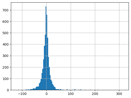
Not perfect agreement (median bias due to different input raster resolution/projection for DEM grid and EGM96 grid, plus nearest neighbor sampling), but at least we’re comparing apples to apples, with both elevations representing height above ellipsoid

Notes on sampling coarse rasters or noisy rasters at integer pixel locations

• The rasterio approach is efficient, but it uses “nearest neighbor” approach to extract the elevation value for the grid cell that contains the point, regradless of where the point falls within the grid cell (center vs. corner)

• But our grid cells can be big (~90x90 m for the global DEM data used here), so if point is near the corner of a pixel on steep slope, the pixel value it might not be representative.

• A better approach is to use bilinear or bicubic sampling, to interpolate the elevation value at the point coordinate using pixel values within some neighborhood around the point, (e.g. 2x2 window for bilinear, 4x4 window for cubic)

• Other approaches using stats for raster values within some radius of the point location (e.g., median elevation of pixels within 300 m of the point)

  • https://www.earthdatascience.org/courses/earth-analytics-python/lidar-remote-sensing-uncertainty/extract-data-from-raster/

  • https://pysal.org/scipy2019-intermediate-gds/deterministic/gds2-rasters.html#getting-values-at-cells

  • https://github.com/uw-cryo/raster_sampling

Extra Credit: Compute stats for circular buffer polygon around each GLAS point using Zonal Statistics

• Buffer with width of 3x the DEM resolution (in meters) and compare with the nearest neighbor values from rasterio sample above

buff_width = src_proj.res[0]*3
buff_width

206.24538555360294

#Create new GeoDataSeries of buffered polygons
glas_gdf_utm_wa_buff = glas_gdf_utm_wa.buffer(buff_width)
glas_gdf_utm_wa_buff

467      POLYGON ((420274.855 5126989.811, 420273.862 5...
468      POLYGON ((420251.930 5127162.809, 420250.937 5...
469      POLYGON ((420229.002 5127335.473, 420228.009 5...
470      POLYGON ((420114.287 5128191.352, 420113.293 5...
471      POLYGON ((420091.581 5128362.681, 420090.588 5...
                               ...                        
65068    POLYGON ((426378.231 5138031.192, 426377.238 5...
65069    POLYGON ((426350.848 5137859.495, 426349.855 5...
65070    POLYGON ((426295.694 5137516.106, 426294.701 5...
65071    POLYGON ((426267.999 5137344.413, 426267.006 5...
65072    POLYGON ((426240.302 5137172.610, 426239.309 5...
Length: 5298, dtype: geometry

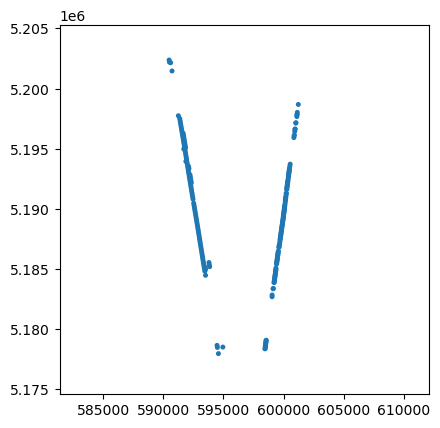
ax = glas_gdf_utm_wa_buff.plot()

#Zoom in, these are circles (buffered polygon around points)
ax = glas_gdf_utm_wa_buff.plot()
ax.set_xlim(581385.0, 612105.0)
ax.set_ylim(5174595.0, 5205315.0)

(5174595.0, 5205315.0)

#Define relevant stats for our sampling
stats=['count', 'min', 'max', 'median', 'std']

#Compute zonal stats for buffered circles around each point using rasterstats
#Note: this could require a few minutes
#https://pythonhosted.org/rasterstats/rasterstats.html
glas_zonal_stats = rasterstats.zonal_stats(glas_gdf_utm_wa_buff, wa_ma, \
                                           affine=wa_ma_transform, nodata=src_proj.nodata, stats=stats)

glas_zonal_stats[0:5]

[{'count': 0, 'min': None, 'max': None, 'median': None, 'std': None},
 {'count': 0, 'min': None, 'max': None, 'median': None, 'std': None},
 {'count': 0, 'min': None, 'max': None, 'median': None, 'std': None},
 {'min': -1.0,
  'max': 3.0,
  'count': 4,
  'std': 1.4142135623730951,
  'median': 1.0},
 {'min': -1.0,
  'max': 11.0,
  'count': 14,
  'std': 2.8437184624849117,
  'median': 1.5}]

#Create a dataframe from the list of dict objects, using original index
glas_zonal_stats_df = pd.DataFrame(glas_zonal_stats, index=glas_gdf_utm_wa_buff.index)
glas_zonal_stats_df

	count	min	max	median	std
467	0	NaN	NaN	NaN	NaN
468	0	NaN	NaN	NaN	NaN
469	0	NaN	NaN	NaN	NaN
470	4	-1.0	3.0	1.0	1.414214
471	14	-1.0	11.0	1.5	2.843718
...	...	...	...	...	...
65068	0	NaN	NaN	NaN	NaN
65069	0	NaN	NaN	NaN	NaN
65070	0	NaN	NaN	NaN	NaN
65071	0	NaN	NaN	NaN	NaN
65072	0	NaN	NaN	NaN	NaN

5298 rows × 5 columns

glas_gdf_utm_wa['buff_med_vs_rio_sample'] = glas_gdf_utm_wa['dem_rio_sample'] - glas_zonal_stats_df['median']
glas_gdf_utm_wa['buff_med_std'] = glas_zonal_stats_df['std']

/srv/conda/envs/notebook/lib/python3.10/site-packages/geopandas/geodataframe.py:1443: SettingWithCopyWarning: 
A value is trying to be set on a copy of a slice from a DataFrame.
Try using .loc[row_indexer,col_indexer] = value instead

See the caveats in the documentation: https://pandas.pydata.org/pandas-docs/stable/user_guide/indexing.html#returning-a-view-versus-a-copy
  super().__setitem__(key, value)
/srv/conda/envs/notebook/lib/python3.10/site-packages/geopandas/geodataframe.py:1443: SettingWithCopyWarning: 
A value is trying to be set on a copy of a slice from a DataFrame.
Try using .loc[row_indexer,col_indexer] = value instead

See the caveats in the documentation: https://pandas.pydata.org/pandas-docs/stable/user_guide/indexing.html#returning-a-view-versus-a-copy
  super().__setitem__(key, value)

glas_gdf_utm_wa['buff_med_vs_rio_sample'].hist(bins=128)

<Axes: >

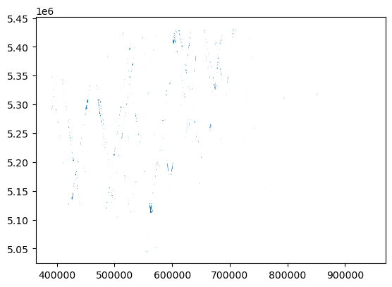
f, axa = plt.subplots(1, 2, figsize=(10,3))
glas_gdf_utm_wa.plot(ax=axa[0], column='buff_med_vs_rio_sample', vmin=-30, vmax=30, cmap='RdBu', s=2, legend=True)
axa[0].set_title('Rasterio sample minus buffered zonal stats')
glas_gdf_utm_wa.plot(ax=axa[1], column='buff_med_std', s=2, vmin=0, vmax=80, legend=True);
axa[1].set_title('Buffered zonal stats std')

Text(0.5, 1.0, 'Buffered zonal stats std')

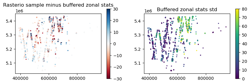
Greatest disagreement is over mountainous areas, where observed std within each ~420 m diameter sample is relatively high

Extra Credit: Do the GLAS points provide a good sample of the observed WA state hypsometry?

• Hypsometry is just total area in different elevation bins (https://en.wikipedia.org/wiki/Hypsometry)

• Plot histogram for your clipped WA DEM

• Plot the histogram of your glas sites on the same axes using the same bins

#Student Exercise

Part 4: Zonal Stats

Which sections of WA highways are surrounded by the steepest slopes?

• Requires sampling a derived DEM product (slope) around Polyline objects (highways)

• This is important for geohazards (rockfall, avalanches)

• You can probably make an informed guess here based on knowledge of the terrain and WA highway network

• Note that in practice, you would want to higher resolution DEM with higher accuracy (e.g., DTM from airborne lidar), but same concept/method applies

Compute surface slope

• Easy to use gdaldem command line utility here (like hillshade generation above) to create a new tif file with slope values

• Can also compute slope directly from our DEM array using np.gradient

slope_fn = os.path.splitext(proj_fn)[0]+'_slope.tif'

#Student Exercise

#Student Exercise

Prepare highway data

• We’ll use some polyline data from Washington State Department of Transportation (WSDOT) here

• https://www.wsdot.wa.gov/mapsdata/geodatacatalog/maps/NOSCALE/DOT_TDO/LRS/sr500kjpg.htm

from datetime import datetime
year = datetime.now().year - 2
#year = 2021

#Link to WA DOT highway data (requires updating each year)
#wa_dot_highway_url = 'https://data.wsdot.wa.gov/geospatial/DOT_TDO/LRS/Historic/500kLRS_2020.zip'
wa_dot_highway_url = f'https://data.wsdot.wa.gov/geospatial/DOT_TDO/LRS/500kLRS_{year}.zip'
#Relative path of the shapefile within the zip archive
wa_dot_highway_shp_fn = f'500k/sr500klines_{year}1231.shp'

Load the shapefile to GeoPandas GeoDataFrame

• We can do this on the fly!

• https://geopandas.readthedocs.io/en/latest/docs/user_guide/io.html#reading-and-writing-files

#Open zip file and contained shapefile on-the-fly with GeoPandas
highways_gdf = gpd.read_file(f'zip+{wa_dot_highway_url}!{wa_dot_highway_shp_fn}')
highways_gdf_utm = highways_gdf.to_crs(src_proj.crs)

highways_gdf.head()

	BARM	EARM	REGION	DISPLAY	RT_TYPEA	RT_TYPEB	LRS_Date	RouteID	StateRoute	RelRouteTy	RelRouteQu	SHAPE_STLe	geometry
0	212.81	213.46	EA	2	US	2	20211231	002	002	None	None	3413.387059	LINESTRING (2077763.828 891111.197, 2077970.07...
1	213.46	242.68	EA	2	US	2	20211231	002	002	None	None	154217.182705	LINESTRING (2080916.017 889804.703, 2082959.44...
2	242.68	243.47	EA	2	US	2	20211231	002	002	None	None	4116.114242	LINESTRING (2217709.066 854913.089, 2219863.05...
3	243.47	253.01	EA	2	US	2	20211231	002	002	None	None	50376.876336	LINESTRING (2221786.174 855269.331, 2222649.58...
4	253.01	255.89	EA	2	US	2	20211231	002	002	None	None	15290.597916	LINESTRING (2271741.605 859012.973, 2277739.38...

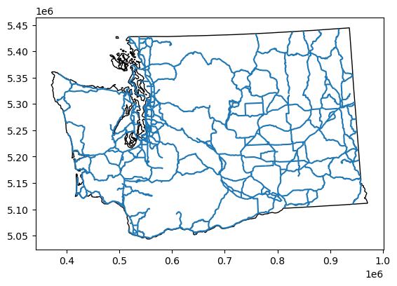
f, ax = plt.subplots()
wa_state.plot(ax=ax, facecolor='none', edgecolor='k')
highways_gdf_utm.plot(ax=ax);

Compute polygons for a 100 m buffer around the polylines

• Remember that the output of buffer is a GeoSeries of Polygons - want to create a new GeoDataFrame and use this as the geometry

• Plot as sanity check. Sample plot shows zoomed in region over I-5 and I-90 interchange, with original lines and buffered polygons in blue

#Student Exercise

#Student Exercise

Now use rasterstats.zonal_stats to compute slope statistics within those polygons

• See the rasterstats documentation: https://pythonhosted.org/rasterstats/manual.html#zonal-statistics

• The docs example uses a shapefile on disk and raster on disk, but we already have our features and raster loaded in memory!

  • Can pass in the GeoDataFrame containing buffered Polygon features instead of a filename

  • Can pass in the slope NumPy array instead of the raster filename, but need to provide the appropriate rasterio dataset transform to the affine keyword

    • Should also pass the appropriate rasterio dataset nodata value

• Compute stats and add the following columns to the highways_gdf_utm geodataframe for each highway segment:

  • mean slope

  • std of slope (a roughness metric)

• Create some plots to visualize

  • If you’re plotting the GeoDataFrame containing the original LINESTRING geometry objects, choose an appropriate linewidth

#Student Exercise

#Student Exercise

#Student Exercise

#Student Exercise

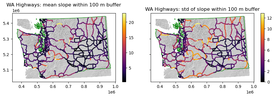
Which section of the highway might you close first during periods of extreme winter weather? ✍️

#Student Exercise

#Student Exercise

Extra Credit

Try one or more of the following:

1. Explore different buffer widths - do your results change?

2. Compute zonal stats for the elevation values (not slope values)

   • Which highway sections cover the greatest elevation range?

3. Compute the slope along the highway polylines, not zonal stats for slope of surrounding terrain

   • Probably want to sample your DEM at points here and compute rise (elevation change) over run (distance between points)

4. Repeat some of the above analysis for WA rivers or watersheds

Extra Credit: explore some spatial functions with xarray-spatial

• We will cover xarray data model in a few weeks, but check out some of the raster/DEM functionality in this new package

Extra Credit: explore some hydrologic functions with RichDEM

• https://github.com/r-barnes/richdem